Overall internal validation

Overview

Data validation is critical at each step of the analysis pipeline. Much of the LFI data validation is based on null tests. Here we present some examples from the current release, with comments on relevant time scales and sensitivity to various systematics. In the 2018 release in addition we perform many test to verify the differences between this and previous release (see Planck-2020-A2).

Null tests approach

Null tests at map level are performed routinely, whenever changes are made to the mapmaking pipeline. These include differences at survey, year, 2-year, half- mission and half-ring levels, for single detectors, horns, horn pairs and full frequency complements. Where possible, map differences are generated in I, Q and U. For this release, we use the Full Focal Plane 10 (FFP10) simulations for comparison. We can use FFP10 noise simulations, identical to the data in terms of sky sampling and with matching time domain noise characteristics, to make statistical arguments about the likelihood of the noise observed in the actual data nulls. In general null tests are performed to highlight possible issues in the data related to instrumental systematic effecst not properly accounted for within the processing pipeline, or related to known changes in the operational conditions (e.g., switch-over of the sorption coolers), or related to intrinsic instrument properties coupled with the sky signal, such as stray light contamination. Such null-tests can be performed by using data on different time scales ranging from 1 minute to 1 year of observations, at different unit levels (radiometer, horn, horn-pair), within frequency and cross-frequency, both in total intensity, and, when applicable, in polarization.

Sample Null Maps

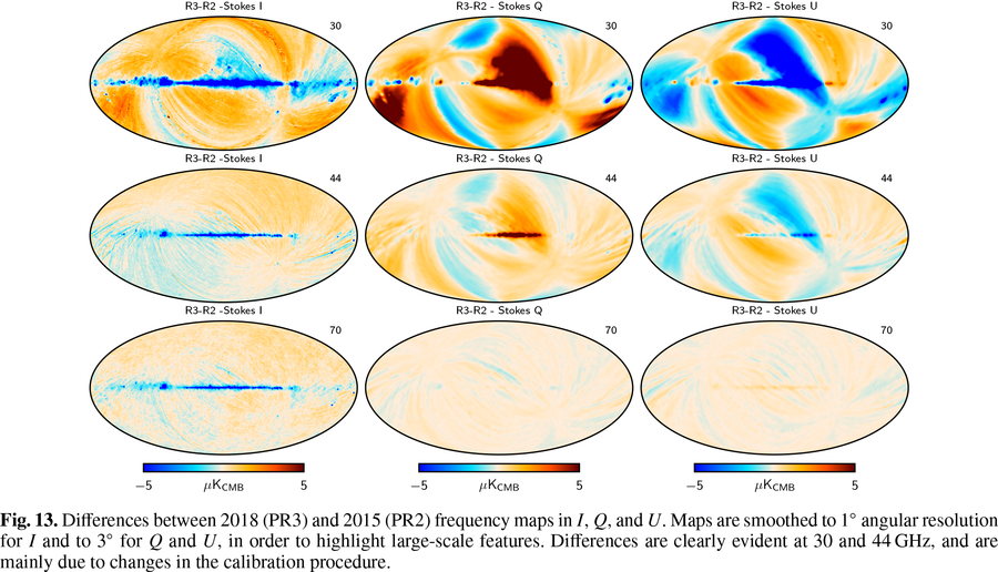
This figure shows difefrences between 2018 and 1015 frequenncy maps in I, Q and U. Large scale differences between the two set of maps are mainly due to changes in the calibration procedure.

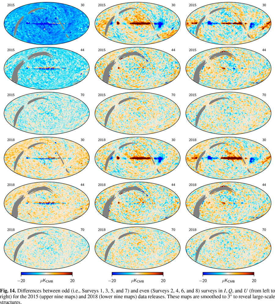
In this figure we consider the set of odd-even survey differences combining all eight sky surveys covered by LFI. These survey combinations optimize the signal-to-noise ratio and highlight large-scale structures. The nine maps on the left show odd-even survey dfferences for the 2015 release, while the nine maps on the right show the same for the 2018 release. The 2015 data show large residuals in I at 30 and 44 GHz that bias the difference away from zero. This effect is considerably reduced in the 2018 release, as expected from the improvements in the calibration process. The I map at 70 GHz also shows a significant improvement. In the polarization maps, there is a general reduction in the amplitude of structures close to the Galactic plane.

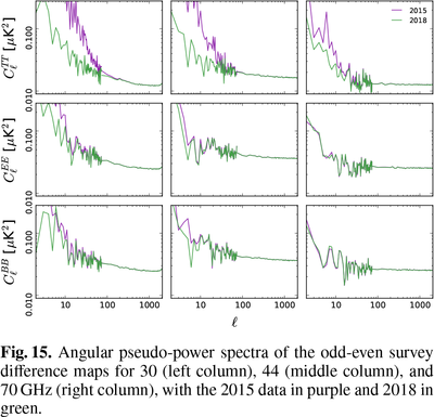
Finally here we shows pseudo-angular power spectra from the oddeven survey dfferences. There is great improvement in 2018 in removing largescale structures at 30 GHz in TT, EE, and somewhat in BB, and also in TT at 44 GHz.

Intra-frequency consistency check

We have tested the consistency between 30, 44, and 70GHz maps by comparing the power spectra in the multipole range around the first acoustic peak. In order to do so, we have removed the estimated contribution from unresolved point source from the spectra. We have then built scatter plots for the three frequency pairs, i.e., 70GHz versus 30 GHz, 70GHz versus 44GHz, and 44GHz versus 30GHz, and performed a linear fit, accounting for errors on both axes. The results reported below show that the three power spectra are consistent within the errors. Moreover, note that the current error budget does not account for foreground removal, calibration, and window function uncertainties. Hence, the observed agreement between spectra at different frequencies can be considered to be even more satisfactory.

70 GHz internal consistency check

We use the Hausman test to assess the consistency of auto- and cross-spectral estimates at 70 GHz. We specifically define the statistic:

[math] H_{\ell}=\left(\hat{C_{\ell}}-\tilde{C_{\ell}}\right)/\sqrt{{\rm Var}\left\{ \hat{C_{\ell}}-\tilde{C_{\ell}}\right\} }, [/math]

where [math]\hat{C_{\ell}}[/math] and [math]\tilde{C_{\ell}}[/math] represent auto- and cross-spectra, respectively. In order to combine information from different multipoles into a single quantity, we define

[math] B_{L}(r)=\frac{1}{\sqrt{L}}\sum_{\ell=2}^{[Lr]}H_{\ell},r\in\left[0,1\right], [/math]

where square brackets denote the integer part. The distribution of B_L(r) converges (in a functional sense) to a Brownian motion process, which can be studied through the statistics s₁=sup_rB_L(r), s₂=sup_r|B_L(r)|, and s₃=∫₀¹B_L²(r)dr. Using the "FFP10" simulations, we derive empirical distributions for all the three test statistics and compare with results obtained from Planck data. We find that the Hausman test shows no statistically significant inconsistencies between the two spectral estimates.