Survey scanning and performance
Contents
[hide]Scanning strategy[edit]
Planck spins at 1 rpm about the symmetry axis of the spacecraft. The boresight of the telescope is 85° from the spin axis. As Planck spins, the instrument beams cover nearly great circles in the sky. The spin axis remains fixed (except for a small drift due to Solar radiation pressure) for between 39 and 65 spins (corresponding to the dwell times given above), depending on which part of its orbit Planck is in. To high accuracy, any one beam covers precisely the same sky between 39 and 65 times. The set of observations made during a period of fixed spin axis pointing is often referred to as a “ring”. This redundancy plays a key role in the analysis of the data, and is an important feature of the scan strategy.


As the Earth and Planck orbit the Sun, the nearly-great circles that are observed rotate about the ecliptic poles. The amplitude of the spin-axis cycloid is chosen so that all beams of both instruments cover the entire sky in one year. In effect, Planck tilts to cover first one Ecliptic pole, then tilts the other way to cover the other pole six months later. If the spin axis stayed exactly on the ecliptic plane, the telescope boresight were perpendicular to the spin axis, the Earth were in a precisely circular orbit, and Planck had only one detector with a beam aligned precisely with the telescope boresight, that beam would cover the full sky in six months. In the next six months, it would cover the same sky, but with the opposite sense of rotation on a given great circle. However, since the spin axis is steered in a cycloid, the telescope is 85° to the spin axis, the focal plane is several degrees wide, and the Earth’s orbit is slightly elliptical, the symmetry of the scanning is (slightly) broken. Thus the Planck beams scan the entire sky exactly twice in one year, but scan only 93% of the sky in six months.
Routine operations[edit]
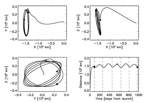
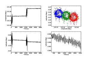
Planck's orbit during routine operations traced a Lissajous path around the L2 point, as shown below.
Routine operations started on 12 August 2009. For convenience, we call an approximately six month period one “survey”, and use that term as an inexact shorthand for one coverage of the sky. Nine numbered “Surveys” are defined precisely in the Table below, which also shows the fraction of the sky covered by all frequencies.
The fourth Survey was shortened somewhat so that the slightly different scanning strategy adopted for Surveys 5–8 (see below) could be started before the Crab nebula, an important polarization calibration source, was observed. The coverage of the fifth Survey is smaller than the others because several weeks of integration time were dedicated to “deep rings” (defined below) covering sources of special importance.

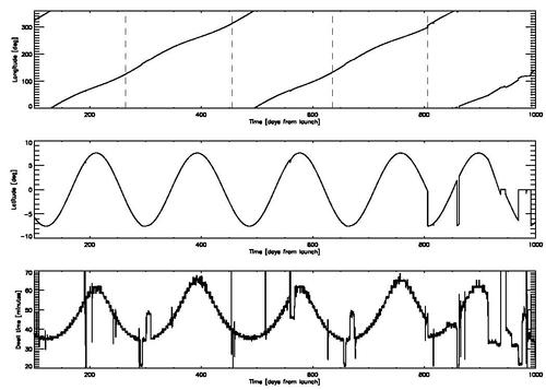
The spin axis was commanded to follow the cycloidal path across the sky in step-wise displacements of 2′ (Fig. 4). To maintain a steady advance of the projected position of the spin axis along the ecliptic plane, the time interval between two manoeuvres varied between 2360 s and 3904 s. The fraction of time used by the manoeuvres themselves (typical duration of five minutes) varied between 6% and 12%, depending on the phase of the cycloid. The data taken during manoeuvres are not used in the analysis. Over the nominal mission, the total reduction of scientific data due to manoeuvres was 9.2%.
The path followed by the Planck spin axis was defined with respect to the Ecliptic plane. It corresponded to a motion in longitude which maintained an anti-Sun pointing (about one degree per day), to which was added a cycloidal motion (precession) of the spin axis around the anti-Sun position (fiducial point). The cycloidal path was defined by the functions
(eq. 1),
(eq. 2),
where λ is the angular distance from the fiducial point in Ecliptic longitude, β the angular distance from the fiducial point in Ecliptic latitude, θ the spin axis precession amplitude, ω the pulsation of the precession, φ its phase, n the parameter which controls the motion direction of the precession, t is the time, and t0 is the first time during the Planck survey at which the fiducial point crosses the Ecliptic longitude =0 line.
The reasons to decide to use such a precession of the spin axis are that: (a) an excursion of the spin axis from the anti-Sun direction is required to fully observe the whole sky (no excursion would leave a large area unobserved around the Ecliptic poles); (b) the precession motion keeps the Sun aspect angle constant during the whole survey, therefore minimizing the thermal constraint variations on the spacecraft.
The following precession parameters were chosen for the scanning strategy of Planck:
- Amplitude θ = 7.5°. (this value is the lowest possible which allows the entire sky to be covered with all detectors).
- n = 1 (anti-clockwise motion as seen from the Sun).
- Pulsation ω = 2π / 6 months (a faster precession was considered, and has interesting advantages, but was not possible given the need to keep a 7.5° amplitude in order to cover the whole sky).
- The phase of the precession was decided according to a set of criteria (in order of importance): (a) respecting the operational constraints; (b) allowing the largest possible angle between two scans on the Crab Nebula (a polarization calibrator); (c) avoiding null dipole amplitude for the whole mission; (d) optimizing the position of the planets in the beginning of the survey and with respect to the feasibility of their recovery; (e) placing the two “deep fields” where Galactic foregrounds are minimum; (f) allowing a reasonable survey margin (i.e. the time allowed to recover lost pointings if a problem occurs). The phase selected was 340° for Surveys 1 to 4, and 250° for Surveys 5 to 8. The cycloid phase was shifted by 90° for Surveys 5–8 to optimize the range of polarization angles on key sources in the combination of Surveys 1–8, thereby helping in the treatment of systematic effects and improving polarization calibration.
The scanning strategy for the second year of Routine Operations (i.e. Surveys 3 and 4) was exactly the same as for the first year, except that all pointings were shifted by 1 arcmin along the cross-scanning direction, in order to provide finer sky sampling for the highest frequency detectors when combining two years of observations.
Routine operations were significantly modified twice more:
- The sorption cooler switchover from the nominal to the redundant unit took place on 11 August 2010, leading to an interruption of acquisition of useful scientific data for about two days (one for the operation itself, and one for re-tuning of the cooling chain).
- The satellite’s rotation speed was increased to 1.4 rpm between 8 and 16 December 2011 for observations of Mars, to measure possible systematic effects on the scientific data linked to the spin rate.
Data were acquired in the normal way during the above two periods, but were not used in the generation of products.
The scientific lifetime of the HFI bolometers ended on 13 January 2012 when the supply of 3He needed to cool them to 0.1K ran out. LFI continued to operate and acquire scientific data until 3 October 2013. On 4 October 2013 Planck ended its routine operations, after executing its last observation of the Crab Nebula, and started its decommissioning activities. On 19 October 2013, the sorption cooler and the two instruments (LFI and HFI) were switched off. The final command to the Planck satellite was sent on 23 October 2013, marking the end of operations.
Add something regarding the final orbit.
Operations were extremely smooth throughout the mission. The total observation time lost due to a few anomalies is about 5 days, spread over the 15.5 months of the nominal mission.
The figure below shows the actual path of the spin axis of Planck during its entire lifetime.
Sky coverage[edit]
As an example, the maps below exhibits the progress of sky coverage during the first months of survey (black colour = unobserved areas).
- HFI 353-GHz integration time after <i
After 1 month
After 2 months
After 3 months
After 4 months
After 5 months
After 6 months
After 7 months
After 8 months
After 9 months
After 10 months
After 11 months
After 12 months


A dynamic visualization of sky coverage by the Planck scanning strategy can be found here and here.
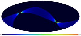
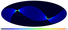
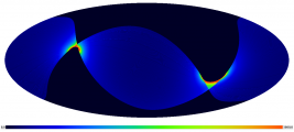
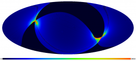
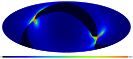
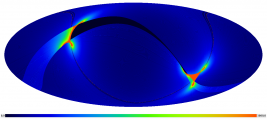
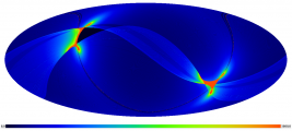
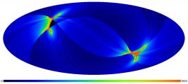
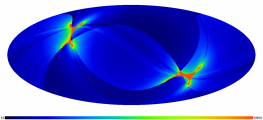
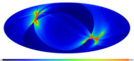
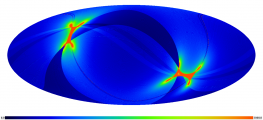
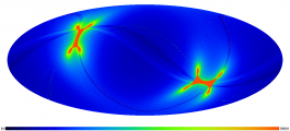
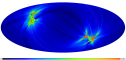
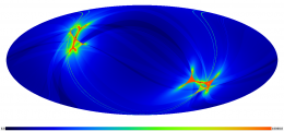
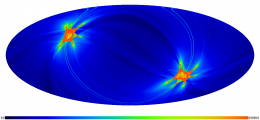
As an additional example, the following figures illustrate the distribution of integration time over the sky for the nominal and “0.1-K” (i.e., until the 3He ran out, see Table) missions, for the 353-GHz frequency channel.
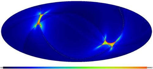
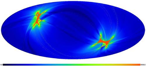
The total integration time after the end of HFI operations (January 2012) is shown in the following maps. Units are seconds per square degree, normalized to one detector, for all maps. The projection is full-sky Mollweide centred on the Galactic centre.
- Integration time after the end of HFI operations (January 2012). The units here are seconds per square degree, normalized to one detector.

HFI 100 GHz 1,4

HFI 100 GHz 2,3

HFI 143 GHz 1-4
HFI 143 GHz 5-8

HFI 217 GHz 1-4

HFI 217 GHz 5-8

HFI 353 GHz

HFI 545 GHz / 857 GHz
LFI-25 (44 GHz)
LFI 30 GHz


Special Observations[edit]
During routine scanning, the Planck instruments naturally observe objects of special interest for calibration. These include Mars, Jupiter, Saturn, Uranus, Neptune, and the Crab nebula. Different types of observations of these objects were performed, as summarised below.
- Normal scans on solar system objects and the Crab nebula. The complete list of observing dates for these objects can be found in Planck Collaboration (2013).
- “Deep rings”. These special scans are performed on observations of Jupiter and the Crab nebula from January 2012 onward. They comprise deeply and finely sampled (step size 0.′5) observations with the spin axis along the Ecliptic plane, lasting typically two to three weeks. Since the Crab is crucial for calibration of both instruments, the average longitudinal speed of the pointing steps was increased before scanning the Crab, to improve operational margins and ease recovery in case of problems.
- “Drift scans”. These special observations are performed on Mars, making use of its proper motion. They allow finely-sampled measurements of the beams, particularly for HFI. The rarity of Mars observations during the mission gives them high priority.
Below is a list of these observations, with the deep rings (Jupiter and the Crab) and drift scans (Mars only) in boldface.
- Crab: 16-22 September 2009
- Mars: 17-29 October 2009
- Jupiter: 25 October – 1 November 2009
- Neptune: 1-8 November 2009
- Uranus: 6-16 December 2009
- Saturn: 2-8 January 2010
- Crab: 6-12 March 2010
- Mars: 9-18 April 2010
- Neptune: 15-23 May 2010
- Saturn: 13-22 June 2010
- Uranus: 27 June – 5 July 2010
- Jupiter: 1-9 July 2010
- Crab: 15-21 September 2010
- Neptune: 3-11 November 2010
- Jupiter: 9-18 December 2010
- Uranus: 12-21 December 2010
- Saturn: 15-22 January 2011
- Crab: 7-12 March 2011
- Neptune: 18-26 May 2011
- Saturn: 30 June - 9 July 2011
- Uranus: 3-11 July 2011
- Jupiter: 9-15 August 2011
- Crab: 10-18 September 2011 (performed with the 250° phase cycloidal strategy)
- Crab: 20-23 September 2011 (performed with the 340° phase cycloidal strategy)
- Mars: 8-16 December 2011 ("drift scan", Mars allowed to move through the Planck focal plane via its proper motion)
- Mars: 17-26 December 2011 (normal scanning)
- Jupiter: 8-30 January 2012 (deep ring)
- Crab: 26 February - 16 March 2012 (deep ring)
- Jupiter: 1-14 September 2012 (deep ring)
- Crab: 14 September - 1 October 2012 (deep ring)
- Neptune: 19-27 November 2012
- Uranus: 24-30 December 2012
- Saturn: 30 January - 5 February 2013
- Jupiter: February 2013 (deep ring)
- Crab: Feb. 28th - March 15th, 2013 (deep ring)
- Neptune: June 4th - June 12th, 2013
- Uranus: July 9-16th, 2013
- Saturn: July 20-26th, 2013
- Crab: Sept. 10th - Oct. 3rd, 2013 (deep ring)
Note that on Sept. 14-16th, 2013, LFI also performed a special dipole calibration observation.
Unplanned events[edit]
The main unplanned events included the following.
- Very minor deviations from the scanning law included occasional (on the average about once every two months) under-performance of the 1-N thrusters used for regular manoeuvres, which implied that the corresponding pointings were not at the intended locations. These deviations had typical amplitudes of 30 arcsec, and had no significant impact on the coverage map.
- The thruster heaters were unintentionally turned off between 31 August and 16 September 2009 (the so-called “catbed” event).
- An operator error in the upload of the on-board command timeline led to an interruption of the normal sequence of manoeuvres and therefore to Planck pointing to the same location on the sky for a period of 29 h between 20 and 21 November 2009 (“the day Planck stood still”). Observations of the nominal scanning pattern resumed on 22 November, and on 23 November a recovery operation was applied to survey the previously missed area. During the recovery period the duration of pointing was decreased to allow the nominal law to be caught up with. As a side effect, the RF transmitter was left on for longer than 24 h, which had a significant thermal impact on the warm part of the satellite.
- As planned, the RF transmitter was initially turned on and off every day in synchrony with the daily visibility window, in order to reduce potential interference by the transmitter on the scientific data. The induced daily temperature variation had a measurable effect throughout the satellite. An important effect was on the temperature of the 4He-JT cooler compressors, which caused variations of the levels of the interference lines that they induce on the bolometer data (Planck HFI Core Team 2011a). Therefore the RF transmitter was left permanently on starting from 25 January 2010 (257 days after launch), which made a noticeable improvement on the daily temperature variations.
- During the coverage period, the operational star tracker switched autonomously to the redundant unit on two occasions (11 January 2010 and 26 February 2010); the nominal star tracker was restored a short period later (3.37 and 12.75 h, respectively) by manual power-cycling. Although the science data taken during this period have normal quality, they have not been used, because the redundant star tracker’s performance is not fully characterized.
For more information, see [1]. For a complete list of operational events, including contigencies, see the POSH (Planck operational state history).
Satellite environment[edit]
The thermal and radiation environment of the satellite during the routine phase is illustrated in the figure below.
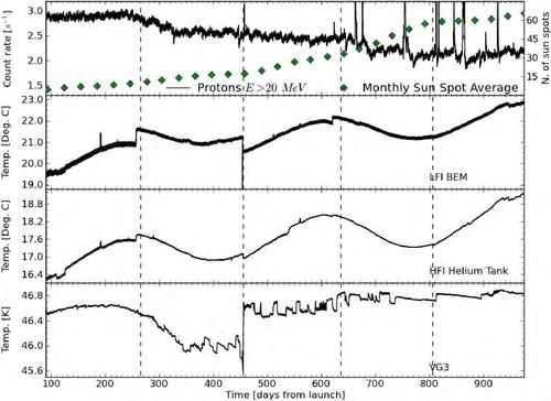
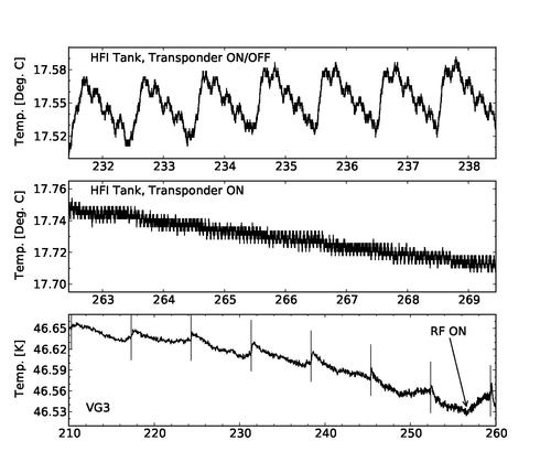
The dominant long-timescale thermal modulation is driven by variations in Solar power absorbed by the satellite in its elliptical orbit around Sun. The thermal environment is sensitive to various satellite operations. For example, before day 257, the communications trans- mitter was turned on only during the daily data transmission period, causing a daily temperature variation clearly visible at all locations in the Service Module (Fig. 6). Some operational events4 had a significant thermal impact as shown in the above figure and detailed in Planck Collaboration (2013): Most notably: a) the “catbed” event between 110 and 126 days after launch; b) the “day Planck stood still” 191 days after launch; c) the sorption cooler switchover (OD 460); d) the change in the thermal control loop (OD 540) of the LFI radiometer electronics assembly box; and e) the spin-up campaign around OD 950.
The sorption cooler dissipates a large amount of power and drives temperature variations at multiple levels in the satellite. The bottom panel of the above figure shows the temperature evolution of the coldest of the three stacked conical structures or V-grooves that thermally isolate the warm service module (SVM) from the cold payload module. Most variations of this structure are due to quasi-weekly power input adjustments of the sorption cooler, whose tube-in-tube heat-exchanger supplying high pressure gas to the 20K Joule-Thomson valve and returning low pressure gas to the compressor assembly is heat-sunk to it. Many adjustments are seen in the roughly three months leading up to switchover. After switchover to the redundant cooler , thermal instabilities were present in the newly operating sorption cooler, which required frequent adjustment, until they reduced significantly around day 750.
The figure also shows the radiation environment history. As Planck started operations, Solar activity was extremely low, and Galactic cosmic rays (which produce sharp “glitches” in the HFI bolometer signals) were more easily able to enter the heliosphere and hit the satellite. As Solar activity increased the cosmic ray flux measured by the onboard standard radiation environment monitor (SREM; Planck Collaboration 2013) decreased correspondingly, but Solar flares increased.
Satellite pointing performance[edit]
Redundant star trackers on board Planck (co-aligned within 0.2° with the instrument field-of-view) provide absolute attitude mea- surements at a frequency of 8 Hz. These measurements are used by the attitude control computer on board Planck to execute the commanded reorientations of the satellite. The star-tracker data were further reprocessed daily on the ground, to provide the following.
- Filtered attitude information at afrequency of 4Hz during the stable observation periods. The filtering algorithm basically suppresses high-frequency components of the measurement noise (i.e., at frequencies well above the nutation frequency);
- Reconstructed attitude parameters averaged over each spin period (60 s) and each stable observation period (or dwell, typically of 50 min length).
The result was a daily attitude history file (AHF), which contained the filtered attitude of the three coordinate axes based on the star trackers every 0.125 s during stable observations (“rings”) and every 0.25 s during re-orientation slews. The production of the AHF was the first step in the determination of the pointing of each detector on the sky. The attitude data during the periods that the satellite is slewing are not filtered on the ground and are therefore much noisier.
The AHF was used by the data processing centres to estimate the location of each detector beam with respect to the satellite reference frame, based mainly on observations of planets (as described in Planck HFI Core Team 2011a).
Planck rotates about its principal axis of inertia at 1 rpm, with a precision of ±0.1% (see the figure).
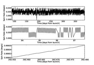
The observed variation of the spin rate was very systematic due to the following operational features.
- The thruster used for a manoeuvre is selected depending on whether the spin rate preceding the manoeuvre is below or above its nominal value. Each thruster has a slightly different “minimum thrust level”, which determines the spin rate actually achieved. Therefore, the spin rate after each manoeuvre will toggle between two different spin rate states which bound the nominal value. If one of these states is very close to the nominal value, drift during the dwell period (see next item) could cause it to change from one side to the other of the nominal value, and thus to toggle on the next manoeuvre to a “third” spin rate state.
- Within a dwell period, the spin rate drifts slightly (typically 10−6 deg s−1 per minute) due to residual torques on the satellite, caused by solar radiation pressure and exhaust of helium from the dilution cooler system.
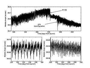
The principal axis of inertia, about which Planck rotates, is off- set from the geometric axis by ∼28.6′ (see the figure). The time evolution of the measured offset angle shows a long-timescale variation which is clearly linked to the seasonal power input vari- ations on the solar array; this effect is not a real variation of the offset angle but is instead due to a thermoelastic deformation of the SVM panel that holds the star trackers (However, it appears as real in the filtered attitude). Other thermoelastic deformations that give rise to similar effects are related to specific operations which have a thermal impact (see Fig. 10). The dominant (false) offset angle variation before 25 January 2010 is due to the daily thermal impact of the RF transponder being switched on and off, and after that date it is related to thermal control cycles in electronic units located near the star trackers; the peak-to-peak amplitude of the effect is of order 0.15′ before and 0.08′ after 25 January. These effects can be correlated to the temperature of the units responsible. They easily mask the real variation of the offset angle, which is due to gradual depletion of the fuel and helium tanks, and is of order 2.5′′ per month
(The variation is approximately 5′ per 50 kg of fuel expended. About 170 g month−1 are expended in scanning manoeuvres and about 50 g in each orbital maintenance manoeuvre, currently performed once every 8 weeks. Approximately 215 g month−1 of helium are vented to space by the HFI dilution cooler.)
. This real variation of the wobble causes a corresponding change over time of the radius of the circle which each detector traces on the sky.
As described in Tauber et al. (2010a), Planck’s spin axis is displaced by 2′ approximately every 50 min. A typical sequence of manoeuvres and dwells is illustrated below.
Each manoeuvre is carried out as a sequence of three thrusts spaced over three minutes (1st impulse – two minutes wait – 2nd impulse – one minute wait – 3rd impulse), designed to cancel nutation as much as possible. Each manoeuvre lasts an average of about 220 s, as defined by on-board software mode transitions9, which are used on the ground to trigger the end and start times of attitude filtering.
The pointing achieved after each reorientation is of course not exactly the commanded one; the difference, which varies between 2 and 8′′ during the coverage period, is shown in Fig. 12.
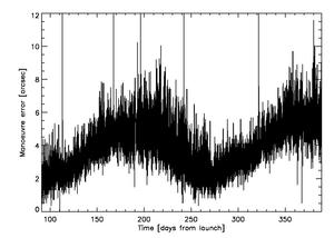
This variation is systematically related to the duration of the dwell preceding the manoeuvre, since the preceding pointing drifts due to solar radiation pressure, and the angular amplitude of the following manoeuvre changes correspondingly. The thrust sequence required for each manoeuvre is computed on-board based on the known mass properties of the satellite and known thruster response functions; the error made on each manoeuvre is mainly driven by the (imperfect) on-board knowledge of these properties, and therefore depends systematically on the amplitude of the manoeuvre. On very few occasions (visible in Fig. 12), the thruster sequence performance did not execute as planned, and resulted in a much larger manoeuvre error.
Although the thruster sequence is designed to damp nutation, it does not do so perfectly. The peak amplitude of the residual nutation is typically 3′′ and does not vary significantly in time (see Fig. 13).
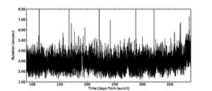
The period of the nutation is 5.425 ± 0.010 min, determined by the inertial properties of the satellite. Neither the amplitude nor the period of the nutation are observed to drift during a dwell period.
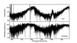
The last major characteristic of pointing within dwells is the drift due to solar radiation pressure. The total amplitude of the drift within each dwell varies between 5 and 12′′, depending on the duration of each dwell (see Fig. 14). The rate of drift varies between 4 and 10′′ h−1, weakly correlated with the Solar Aspect Angle (which varies by very small amounts throughout the mission).
The pointing characteristics at AHF level are summarized in the table below.

A detailed description of the AHF algorithm and its performance in flight can be found in Tuttlebee & Gienger 2012[2].
Improvements on the AHF[edit]
Early on it was realized that there were some problems with the pointing solutions. First, the attitude determination during slews was poorer than during periods of stable pointing. Second, the solutions were affected by thermoelastic deformations in the satellite driven by temperature variations resulting from imperfect thermal control loops, the sorption cooler, and the thermally- driven transfer of helium from one tank to another.
A significant effort was made to improve ground processing capability to address the above issues. As a result, three different versions of the attitude history were produced for the whole mission:
- the AHF, based on an optimized version of the initial (pre-launch) algorithm;
- the Gyro-based attitude history hile (GHF), based on an algorithm that uses, in addition to the star tracker data, angular rate measurements derived from the on-board fibre-optic gyro (note that it was not initially planned to use its data for computation of the attitude over the whole mission)
- the Dynamical attitude history file (DHF), based on an algorithm that uses the star tracker data in conjunction with a dynamical model of the satellite, and which accounts for the existence of disturbances at known sorption cooler operation frequencies.
Both the GHF and DHF algorithms significantly improve the recovery of attitude during slews. Due to the deadlines involved, the optimised AHF algorithm has been used in the production of the Planck products. Use the improved algorithms could enable the use of the scientific data acquired during slews (9.2% of the total).
Tuttlebee & Gienger 2012[2] also includes an analysis of the performance of GHF and DHF.
References[edit]
- Jump up ↑ Planck early results. I. The Planck mission, Planck Collaboration I, A&A, 536, A1, (2011).
- ↑ Jump up to: 2.02.1 Planck On-Ground Attitude Estimation Algorithms, Tuttlebee, M., & Gienger, G. 2012
revolutions per minute
(Planck) High Frequency Instrument
(Planck) Low Frequency Instrument
Operation Day definition is geometric visibility driven as it runs from the start of a DTCP (satellite Acquisition Of Signal) to the start of the next DTCP. Given the different ground stations and spacecraft will takes which station for how long, the OD duration varies but it is basically once a day.
Space Radiation Environment Monitor
Service Module
Attitude History File