Difference between revisions of "HFI design, qualification, and performance"
| Line 795: | Line 795: | ||
== System (Ken) == | == System (Ken) == | ||
===List of systematics=== | ===List of systematics=== | ||
| + | |||
| + | {{:HFI-Validation#Expected systematics and tests (bottom-up approach)}} | ||
==Summary== | ==Summary== | ||
Revision as of 06:06, 19 October 2012
The inversion of HFI data requires that one knows how the instrument selects photons, how these photons are transformed in data transmitted by telemetry and what spurious signals are added in this process.
Contents
HFI high level description and Architecture[edit]
(Lamarre/Pajot) Should be short, understandable and point through links to the relevant sections and papers.
Cryogenics[edit]
(F .Pajot)
Dilution[edit]
(including PIDs)
The HFI 3He-4He dilution cooler produces temperatures of 0.1 K for the bolometers through the dilution of 3He into 4He and 1.4 K through JT expansion of the 3He and 4He mixture. The dilution cooler is described in detail in [Planck early results. II. The thermal performance of Planck, 2.3.3. Dilution cooler].
The dilution was operated with flows set to the minimum available value, and provided a total lifetime of 30.5 months, exceeding the nominal lifetime of 16 months by 14.5 months. The dilution stage was stabilized by a PID control with a power comprised between 20 and 30 nW providing a temperature near 101 mK. The bolometer plate was stabilized at 102.8 mK with a PID power around 5 nW [fig. 100mK_stability.png].
(here a few lines of 100 mK boloplate stability)
Detailed of the in-flight performance of the dilution cooler can be found in [Planck early results. II. The thermal performance of Planck, 4.4. Dilution cooler]
4K J-T cooler[edit]
(including PIDs for details links to the early cryogenic paper (need to add data ?))
The HFI 4K J-T cooler produces a temperature of 4K for the HFI 4K stage and optics and the precooling of the dilution gases. Full description of the 4K cooler can be found in [Planck early results. II. The thermal performance of Planck, 2.3.2. 4He-JT cooler].
The 4K cooler was operated without interruption during all the survey phase of the mission. It is still in operation as it also provides the cooling of the optical reference loads of the LFI. The 4K PID stabilizing the temperature of the HFI optics is regulated at 4.81 K using a power around 1.8 mW [fig. 4K -A VENIR-].
(here a few lines of 4K stability, including compressors operation)
Details on the in-flight performance of the dilution cooler can be found in [Planck early results. II. The thermal performance of Planck, 4.3. 4He-JT cooler]

Cold optics[edit]
(Lamarre)
Horns,lenses[edit]
links to Peter's paper
filters, band[edit]
Includes Locke's very detailed document.
Detection chain[edit]
(Francesco Piacentini)
Bolometers[edit]
JFETs[edit]
Readout[edit]
Data compression[edit]
Time response.[edit]
The HFI bolometers and readout electronics have a finite response time to changes in incident optical power. The bolometers are thermal detectors of radiation whose response time is determined by the thermal circuit defined by the heat capacity of the detector and thermal conductivity.
Due to Planck's nearly constant scan rate, the time response is degenerate with the optical beam. However, because of the long time scale effects present in the time response, the time response is deconvolved from the data in the processing of the HFI data (see TOI processing).
The time response of the HFI bolometers and readout electronics is modeled as a Fourier domain transfer function (called the LFER4 model) consisting of the product of an bolometer thermal response and an electronics response .
LFER4 model[edit]
If we write the input signal (power) on a bolometer as the bolometer physical impedance can be written as: where is the angular frequency of the signal and is the complex intrinsic bolometer transfer function. For HFI the bolometer transfer function is modelled as the sum of 4 single pole low pass filters: The modulation of the signal is done with a square wave, written here as a composition of sine waves of decreasing amplitude: where we have used the Euler relation and is the angular frequency of the square wave. The modulation frequency is and was set to Hz in flight. This signal is then filtered by the complex electronic transfer function . Setting: we have: This signal is then sampled at high frequency (). is one of the parameters of the HFI electronics and corresponds to the number of high frequency samples in each modulation semi-period. In order to obtain an output signal sampled every seconds, we must integrate on a semiperiod, as done in the HFI readout. To also include a time shift , the integral is calculated between and (with period of the modulation). The time shift is encoded in the HFI electronics by the parameter , with the relation .
After integration, the -sample of a bolometer can be written as where
The output signal in equation eqn:output can be demodulated (thus removing the ) and compared to the input signal in equation bol_in. The overall transfer function is composed of the bolometer transfer function and the effective electronics transfer function, :
The shape of is obtained combining low and high-pass filters with Sallen Key topologies (with their respective time constants) and accounting also for the stray capacitance low pass filter given by the bolometer impedance combined with the stray capacitance of the cables. The sequence of filters that define the electronic band-pass function are listed in table table:readout_electronics_filters.
Parameters of LFER4 model[edit]
The LFER4 model has are a total of 10 parameters(,,,,,,,,,) 9 of which are independent, for each bolometer. The free parameters of the LFER4 model are determined using in-flight data in the following ways:
- is fixed at the value of the REU setting.
- is measured during the QEC test during CPV.
- , , , are fit forcing the compactness of the scanning beam.
- , , are fit by forcing agreement of survey 2 and survey 1 maps.
- The overall normalization of the LFER4 model is forced to be 1.0 at the signal frequency of the dipole.
The details of determining the model parameters are given in (reference P03c paper) and the best-fit parameters listed here in table table:LFER4pars.
HFI electronics filter sequence[edit]
| Filter | Parameters | Function |
|---|---|---|
| 0. Stray capacitance low pass filter | ||
| 1. Low pass filter | k nF |
|
| 2. Sallen Key high pass filter | k |
3 |
| 3. Sign reverse with gain | ||
| 4. Single pole low pass filter with gain | k nF |
|
| 5. Single pole high pass filter coupled to a Sallen Key low pass filter | k k nF k F |
| Bolometer | (s) | (s) | (s) | (s) | (s) | |||||
| 100-1a | 0.392 | 0.01 | 0.534 | 0.0209 | 0.0656 | 0.0513 | 0.00833 | 0.572 | 0.00159 | 0.00139 |
| 100-1b | 0.484 | 0.0103 | 0.463 | 0.0192 | 0.0451 | 0.0714 | 0.00808 | 0.594 | 0.00149 | 0.00139 |
| 100-2a | 0.474 | 0.00684 | 0.421 | 0.0136 | 0.0942 | 0.0376 | 0.0106 | 0.346 | 0.00132 | 0.00125 |
| 100-2b | 0.126 | 0.00584 | 0.717 | 0.0151 | 0.142 | 0.0351 | 0.0145 | 0.293 | 0.00138 | 0.00125 |
| 100-3a | 0.744 | 0.00539 | 0.223 | 0.0147 | 0.0262 | 0.0586 | 0.00636 | 0.907 | 0.00142 | 0.00125 |
| 100-3b | 0.608 | 0.00548 | 0.352 | 0.0155 | 0.0321 | 0.0636 | 0.00821 | 0.504 | 0.00166 | 0.00125 |
| 100-4a | 0.411 | 0.0082 | 0.514 | 0.0178 | 0.0581 | 0.0579 | 0.0168 | 0.37 | 0.00125 | 0.00125 |
| 100-4b | 0.687 | 0.0113 | 0.282 | 0.0243 | 0.0218 | 0.062 | 0.00875 | 0.431 | 0.00138 | 0.00139 |
| 143-1a | 0.817 | 0.00447 | 0.144 | 0.0121 | 0.0293 | 0.0387 | 0.0101 | 0.472 | 0.00142 | 0.00125 |
| 143-1b | 0.49 | 0.00472 | 0.333 | 0.0156 | 0.134 | 0.0481 | 0.0435 | 0.27 | 0.00149 | 0.00125 |
| 143-2a | 0.909 | 0.0047 | 0.0763 | 0.017 | 0.00634 | 0.1 | 0.00871 | 0.363 | 0.00148 | 0.00125 |
| 143-2b | 0.912 | 0.00524 | 0.0509 | 0.0167 | 0.0244 | 0.0265 | 0.0123 | 0.295 | 0.00146 | 0.00125 |
| 143-3a | 0.681 | 0.00419 | 0.273 | 0.00956 | 0.0345 | 0.0348 | 0.0115 | 0.317 | 0.00145 | 0.00125 |
| 143-3b | 0.82 | 0.00448 | 0.131 | 0.0132 | 0.0354 | 0.0351 | 0.0133 | 0.283 | 0.00161 | 0.000832 |
| 143-4a | 0.914 | 0.00569 | 0.072 | 0.0189 | 0.00602 | 0.0482 | 0.00756 | 0.225 | 0.00159 | 0.00125 |
| 143-4b | 0.428 | 0.00606 | 0.508 | 0.00606 | 0.0554 | 0.0227 | 0.00882 | 0.084 | 0.00182 | 0.00125 |
| 143-5 | 0.491 | 0.00664 | 0.397 | 0.00664 | 0.0962 | 0.0264 | 0.0156 | 0.336 | 0.00202 | 0.00139 |
| 143-6 | 0.518 | 0.00551 | 0.409 | 0.00551 | 0.0614 | 0.0266 | 0.0116 | 0.314 | 0.00153 | 0.00111 |
| 143-7 | 0.414 | 0.00543 | 0.562 | 0.00543 | 0.0185 | 0.0449 | 0.00545 | 0.314 | 0.00186 | 0.00139 |
| 217-5a | 0.905 | 0.00669 | 0.0797 | 0.0216 | 0.00585 | 0.0658 | 0.00986 | 0.342 | 0.00157 | 0.00111 |
| 217-5b | 0.925 | 0.00576 | 0.061 | 0.018 | 0.00513 | 0.0656 | 0.0094 | 0.287 | 0.00187 | 0.00125 |
| 217-6a | 0.844 | 0.00645 | 0.0675 | 0.0197 | 0.0737 | 0.0316 | 0.0147 | 0.297 | 0.00154 | 0.00125 |
| 217-6b | 0.284 | 0.00623 | 0.666 | 0.00623 | 0.0384 | 0.024 | 0.0117 | 0.15 | 0.00146 | 0.00111 |
| 217-7a | 0.343 | 0.00548 | 0.574 | 0.00548 | 0.0717 | 0.023 | 0.0107 | 0.32 | 0.00152 | 0.00139 |
| 217-7b | 0.846 | 0.00507 | 0.127 | 0.0144 | 0.0131 | 0.0479 | 0.0133 | 0.311 | 0.00151 | 0.00139 |
| 217-8a | 0.496 | 0.00722 | 0.439 | 0.00722 | 0.0521 | 0.0325 | 0.0128 | 0.382 | 0.00179 | 0.00111 |
| 217-8b | 0.512 | 0.00703 | 0.41 | 0.00703 | 0.0639 | 0.0272 | 0.0139 | 0.232 | 0.00173 | 0.00125 |
| 217-1 | 0.0136 | 0.00346 | 0.956 | 0.00346 | 0.0271 | 0.0233 | 0.00359 | 1.98 | 0.00159 | 0.00111 |
| 217-2 | 0.978 | 0.00352 | 0.014 | 0.0261 | 0.00614 | 0.042 | 0.00194 | 0.686 | 0.0016 | 0.00125 |
| 217-3 | 0.932 | 0.00355 | 0.0336 | 0.00355 | 0.0292 | 0.0324 | 0.00491 | 0.279 | 0.00174 | 0.00125 |
| 217-4 | 0.658 | 0.00135 | 0.32 | 0.00555 | 0.0174 | 0.0268 | 0.00424 | 0.473 | 0.00171 | 0.00111 |
| 353-3a | 0.554 | 0.00704 | 0.36 | 0.00704 | 0.0699 | 0.0305 | 0.0163 | 0.344 | 0.0017 | 0.00125 |
| 353-3b | 0.219 | 0.00268 | 0.671 | 0.00695 | 0.0977 | 0.0238 | 0.0119 | 0.289 | 0.00157 | 0.00111 |
| 353-4a | 0.768 | 0.00473 | 0.198 | 0.00993 | 0.0283 | 0.0505 | 0.00628 | 0.536 | 0.00181 | 0.00125 |
| 353-4b | 0.684 | 0.00454 | 0.224 | 0.0108 | 0.0774 | 0.08 | 0.0149 | 0.267 | 0.00166 | 0.00111 |
| 353-5a | 0.767 | 0.00596 | 0.159 | 0.0124 | 0.0628 | 0.0303 | 0.0109 | 0.357 | 0.00156 | 0.00111 |
| 353-5b | 0.832 | 0.00619 | 0.126 | 0.0111 | 0.0324 | 0.035 | 0.0096 | 0.397 | 0.00166 | 0.00111 |
| 353-6a | 0.0487 | 0.00176 | 0.855 | 0.006 | 0.0856 | 0.0216 | 0.0105 | 0.222 | 0.00199 | 0.00125 |
| 353-6b | 0.829 | 0.00561 | 0.127 | 0.00561 | 0.0373 | 0.0252 | 0.00696 | 0.36 | 0.00228 | 0.00111 |
| 353-1 | 0.41 | 0.000743 | 0.502 | 0.00422 | 0.0811 | 0.0177 | 0.0063 | 0.329 | 0.00132 | 0.00097 |
| 353-2 | 0.747 | 0.00309 | 0.225 | 0.00726 | 0.0252 | 0.0447 | 0.00267 | 0.513 | 0.00154 | 0.00097 |
| 353-7 | 0.448 | 0.0009 | 0.537 | 0.0041 | 0.0122 | 0.0273 | 0.00346 | 0.433 | 0.00178 | 0.00125 |
| 353-8 | 0.718 | 0.00223 | 0.261 | 0.00608 | 0.0165 | 0.038 | 0.00408 | 0.268 | 0.00177 | 0.00111 |
| 545-1 | 0.991 | 0.00293 | 0.00743 | 0.026 | 0.00139 | 2.6 | 0 | 0 | 0.00216 | 0.00111 |
| 545-2 | 0.985 | 0.00277 | 0.0128 | 0.024 | 0.00246 | 2.8 | 0 | 0 | 0.00187 | 0.00097 |
| 545-4 | 0.972 | 0.003 | 0.0277 | 0.025 | 0.000777 | 2.5 | 0 | 0 | 0.00222 | 0.00111 |
| 857-1 | 0.974 | 0.00338 | 0.0229 | 0.025 | 0.00349 | 2.2 | 0 | 0 | 0.00176 | 0.00111 |
| 857-2 | 0.84 | 0.00148 | 0.158 | 0.00656 | 0.00249 | 3.2 | 0 | 0 | 0.0022 | 0.00125 |
| 857-3 | 0.36 | 4.22e-05 | 0.627 | 0.0024 | 0.0111 | 0.017 | 0.002 | 1.9 | 0.00152 | 0.00126 |
| 857-4 | 0.278 | 0.0004 | 0.719 | 0.00392 | 0.00162 | 0.09 | 0.00152 | 0.8 | 0.00149 | 0.000558 |
System (Ken)[edit]
List of systematics[edit]
The overall internal validation of the frequency maps is performed thanks to several tests:
- difference between the PR2 (2015) and PR3 (2018) frequency maps,
- survey difference maps for the PR2 and the PR3 frequency maps,
- spectra of the PR2 and the PR3 data splits,
- comparison of the FFP10 simulations and the PR3 data.
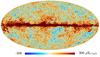
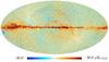
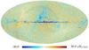
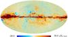
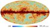
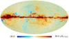
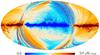
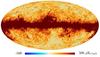
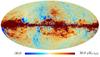
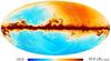
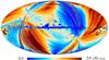
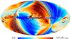
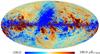
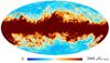
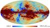
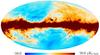
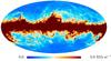
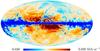
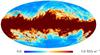
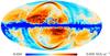
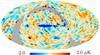
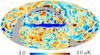
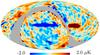
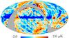
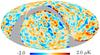
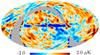
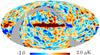
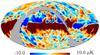
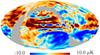
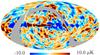
Frequency maps for the PR2 and the PR3 and their difference
This table shows the PR2 and PR3 maps and their differences in I, Q, and U. This table is complementary of the figure in Planck-2020-A3[1] (see detailled explanations there).
| PR2 frequency maps | PR3 frequency maps | difference | |||||||
|---|---|---|---|---|---|---|---|---|---|
| I | Q | U | I | Q | U | I | Q | U | |
| 100 GHz | 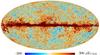
|
|
|
|
|
|
|
|
|
| 143 GHz | 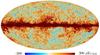
|
|
|
|
|
|
|
|

|
| 217 GHz | 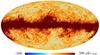
|
|
|
|
|
|
|
|
|
| 353 GHz | 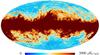
|
|
|
|
|
|
|
|
|
| 545 GHz | 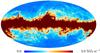
|
. | . | 
|
. | . | 
|
. | . |
| 857 GHz | 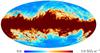
|
. | . | 
|
. | . | 
|
. | . |
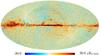
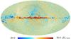
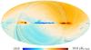
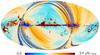
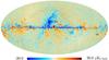
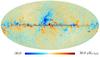
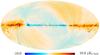
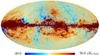
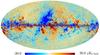
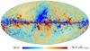
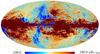
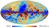
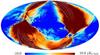
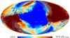
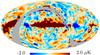
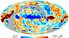
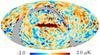
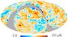
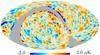
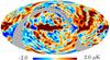
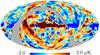
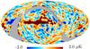
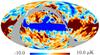
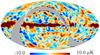
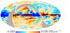
Survey difference maps for the PR2 and the PR3 data
This table shows the PR2 and PR3 survey difference maps ((S1+S3)-(S2+S4))in I, Q, and U. This table is taken from Planck-2020-A3[1] (see detailled explanations there).
| PR2 survey difference maps | PR3 survey difference maps | |||||
|---|---|---|---|---|---|---|
| I | Q | U | I | Q | U | |
| 100 GHz | 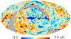
|
|
|
|
|
|
| 143 GHz | 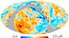
|
|
|
|
|
|
| 217 GHz | 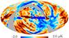
|
|
|
|
|
|
| 353 GHz | 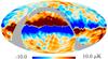
|
|
|
|
|
|
| 545 GHz | 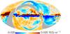
|
. | . | 
|
. | . |
| 857 GHz | 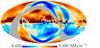
|
. | . | 
|
. | . |
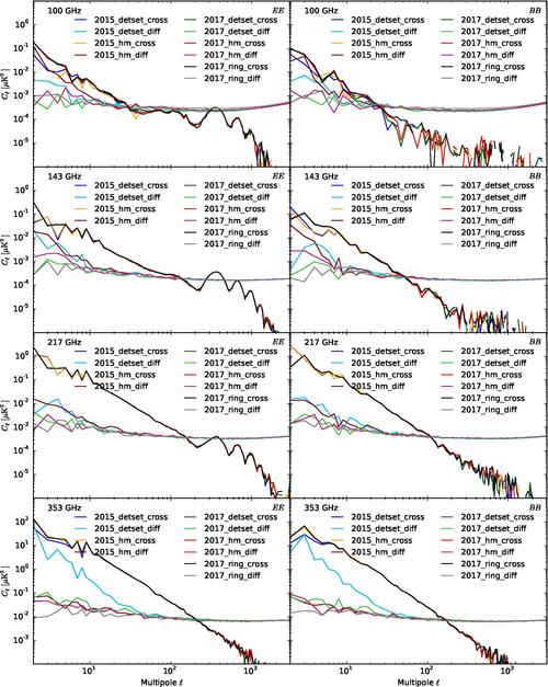
Spectra of the PR2 and the PR3 data splits
This figure shows the EE and BB spectra of the PR2 and PR3 detset, half-mission and rings (for PR3 only) maps at 100, 143, 217, and 353 GHz. The auto-spectra of the difference maps and the cross-spectra between the maps are shown. The sky fraction used here is 43 %. The bins are: bin=1 for ; bin=5 for ; bin=10 for ; bin=20 for ; and bin=100 for . This figure is taken from Planck-2020-A3[1] (see detailled explanations there).
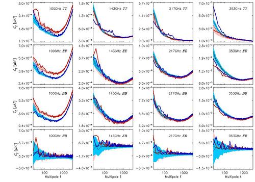
Comparison of the FFP10 simulated noise and systematic residuals and the PR3 data
This figure shows the noise and systematic residuals in TT, EE, BB, and EB spectra, at the three CMB frequencies, for difference maps of the ring (red) and half-mission (blue) null tests binned by . Data spectra are represented by thick lines, and the averages of simulations by thin black lines. For the simulations, we show the 16 % and 84 % quantiles of the distribution with the same colours. This figure is taken from Planck-2020-A3[1] (see detailled explanations there).
References[edit]
- ↑ 1.01.11.21.3 Planck 2018 results. III. High Frequency Instrument data processing and frequency maps, Planck Collaboration, 2020, A&A, 641, A3.
Summary[edit]
(Lamarre) here remind worse sytematics and point to DPC Summary of sucess and limitations. JML. Link to early HFI in flight perf.
(Planck) High Frequency Instrument
(Planck) Low Frequency Instrument
Readout Electronic Unit
Calibration and Performance Verification
Cosmic Microwave background
Data Processing Center