TOI processing
Contents
[hide]Overview[edit]
We describe here how the TOIs are processed in order to be used for map production. They are first corrected for non-linear effects in the ADCs, then processed with a pipeline whose general features are given in the HFI Data Processing paper Planck-2013-VI[1] for PR1 and Planck-2015-A07[2] for PR2. For PR3 (2018 release), the main change with respect to 2015 has been in the selection of data: the last 955 pointings (or rings) have not been used because they have been found to be affected by thermal fluctuations (see Planck-2020-A3[3]).
Detailed explanations of each stage of the TOI processing are given in various papers, referenced in the diagram below (taken from Planck-2020-A3[3]).

Here we give complementary explanations in some detail. The TOI of each bolometer is processed independently of the other bolometers, so as to keep the noise properties as uncorrelated as possible. The pipeline processing involves modifying the TOI itself for the conversion to absorbed power and the correction of glitch tails. It also adds a flag TOI that masks the TOI samples that are not to be projected onto maps for various reasons.
The input TOI consists of the AC-modulated voltage output read out of each bolometer. The input has previously been decompressed, and converted from internal digital units to voltages via a constant factor. The TOI has a regular sampling at the acquisition frequency of facq=(180.373700±0.000050)Hz. There are almost no missing data samples in the TOIs, except for a few hundred samples of 545 and 857 GHz TOIs, which were lost in the on-board compression due to saturation on the Galactic centre crossings.
ADC non-linearity correction[edit]
On-board, the modulated bolometer outputs are sampled 20x during each half-cycle, and the 20 samples are then averaged into the individual samples that are compressed and transmitted to ground. The ADC non-linearity affects the signals before the averaging, and a complicated process is necessary to determine and remove the systematic effects induced by that non-linearity, a process that is further complicated by the 40-Hz parasitics associated with the 4-K cooler drive electronics.
The principles of the correction are detailed in Planck-2015-A07[2]. The correction cannot be done using only the TOI values, but requires ancillary data from ground-based tests and additional tests done during the LFI extension of the mission, when the dilution cooler no longer operated. For this reason, we do not describe here any details that are not already in the paper, since the users should not expect to be able to improve this part of the processing.
The result of this processing is a corrected TOI, always in ADUs, which is then fed to the TOI processing pipeline described below.
General pipeline structure[edit]
The following figure shows how the initial TOI is transformed and how flags are produced.

Output TOIs and products[edit]
A TOI of clean calibrated samples and a combined flag TOI are the outputs of the processing. The clean calibrated TOI is calibrated so as to represent the instantaneous power absorbed by the detector, up to a constant (which will be determined by the mapmaking destriper). It is worth mentioning how the clean calibrated TOI is changed with respect to the input TOI, beyond the basic constant conversion factor from voltage to absorbed power. The demodulation stage allows one to obtain the demodulated bolometer voltage. The nonlinearity correction is a second-order polynomial correction based on the physical but static bolometer model. In order to avoid too much masking after glitches, a glitch tail is subtracted after an occurrence of a glitch in the TOI. The 4-K cooler lines are removed at a series of nine single temporal frequencies. Finally, the temporal response of the bolometer is deconvolved. This affects mostly the high-temporal frequency part of the TOI, although a small but significant low frequency tail (the long time response) is corrected too. Although flagged samples are not projected, their value still influences the valid samples. Hence interpolation procedures introduce some indirect modifications of the TOI. The flag TOI is a combination of flags with an OR logic. Only unflagged data are projected. The exhaustive list of flags is: CompressionError; SSO; UnstablePointing; Glitch; BoloPlateFluctuation; RTS; Jump; and PSBab. A complete qualification of the data is obtained at the ring level. If the TOI shows any anomalous behaviour on a given ring, this ring is discarded from projection. A special TOI is also produced as an input to the beam analysis for Mars, Jupiter, and Saturn.
Examples of clean TOIs[edit]
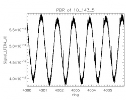
Phase-binned signal (PBR) for six consecutive rings from 4000 to 4005.
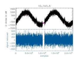
Valid signal (up) and noise (bottom) for two consecutive circles of ring 4000.
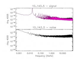
Fourier power spectral density of the first 30 minutes of ring 4005 with signal (top) before (pink) and after (black) deconvolution and with noise (bottom) also shown.
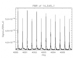
Phase-binned signal (PBR) for six consecutive rings from 4000 to 4005.
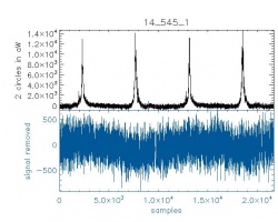
Valid signal (up) and noise (bottom) for two consecutive circles of ring 4000.
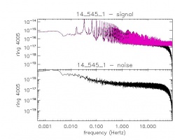
Fourier power spectral density of the first 30 minutes of ring 4005, with signal (top) before (pink) and after (black) deconvolution and with noise (bottom) also shown.


Samples of PBR, TOIs, and PSDs of all detectors are shown in this file.
Trends in the output processing variables[edit]
Here we show trends in the systematic effects that are dealt with in the TOI processing. The full impact of each of them is analysed in the HFI-Validation section.
ADC baseline[edit]
The following figure shows the ADC baseline that is used prior to demodulation (a constant offset is removed for clarity). This baseline is obtained by smoothing on an hour timescale by block-averaging the undemodulated TOI on unflagged samples.

Glitch statistics[edit]
The glitch rate per channel is shown in the figure below. For details, see Planck-2013-X[4]

The percentage of flagged data (mostly due to cosmic rays) at the ring level is shown in these examples. No smoothing was applied and only valid rings are shown.
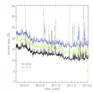
143GHz bolometers.
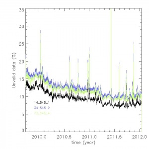
545GHz bolometers.


Percentage of flagged data
The complete set of plots is attached here.
Thermal template for decorrelation[edit]

A simple linear decorrelation is performed using the two "dark" bolometers as a proxy of the bolometer plate temperature. Coupling coefficients were measured during the CPV phase.
4-K cooler lines variability[edit]
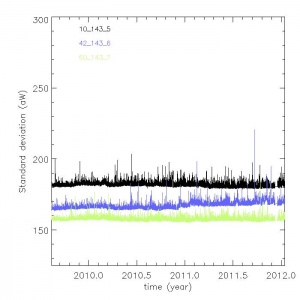
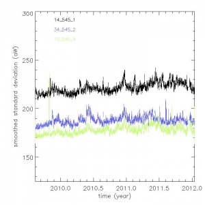
The amplitude of the nine 4-K cooler lines at 10, 20, 30, 40, 50, 60, 70, 80, and 17Hz is shown (in aW) for two bolometers in the following figures. The trend is smoothed over 31 ring values after having discarded measurements done at a ring that is discarded for all bolometers.
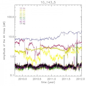
143_5 bolometer.
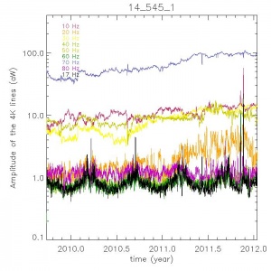
545_1 bolometer.


Amplitude of the nine 4-K cooler lines
The 4-K cooler line coefficients of all bolometers are shown in this file.
The 4-K cooler lines project onto the maps only for a limited fraction of rings, the so-called "resonant rings." This is graphically shown in the following figure. For each ring (fixed pointing period), the spin rate is very stable at about 1rpm. From one ring to another, the spin frequency (shown as diamonds) changes around that value. The sky signal is imprinted at the corresponding spin frequency and its 5400 (60×90) harmonics. If one of the nine 4-K cooler lines happens to coincide with one of the spin frequency harmonics (a resonant ring), it will project a sine-wave systematic onto the maps. The horizontal coloured bars show the zone of influence of a particular 4-K line (labelled on the left side of the plot), when folded around 16.666mHz. When the spin frequency hits one of these zones, we have a resonant ring. The 4-K line coefficient is interpolated for this ring and an estimate of the systematic effect is subtracted from the TOI. Resonant rings are different for different 4-K lines. Note the two-level oscillation pattern of the spin frequency, which is due to the satellite attitude control system.

Jump correction[edit]
A piecewise constant value is removed from the TOI if a jump is detected. An example of a jump is shown in the following figure:

The number of jumps per day (all bolometers included) is shown in this figure:

The jumps are uncorrelated from bolometer to bolometer. The total number of jumps detected in the nominal and full mission is shown below:

Trends in noise and signal[edit]
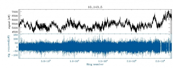
143_5 bolometer.
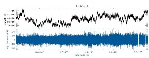
545_1 bolometer.


Signal (top) and noise (bottom) smoothed over 1 minute. All values falling in a discarded ring are not plotted.
The smooth TOIs of all detectors are shown in this file.
Noise stationarity[edit]
This is not the final version but gives a good idea of power spectra at the detector level of noise TOIs. All PSDs can be seen in this file.
The standard deviation per ring corrected for ring duration bias is given here, one per bolometer using only valid rings. No smoothing is applied (except a 31-point smoothing for the 545 and 857 GHz channels), but values for rings discarded for all bolometers (see below) are not used. The standard deviation is computed on samples valid for mapmaking that are also not affected by the Galaxy or the point-sources using the usual flags. Two examples are shown below.
143_5 bolometer.
545_1 bolometer.


Standard deviation per ring
The full series of plots of the Standard deviation of noise TOIs at the ring level is here.
Note the presence for three bolometers of a two-level noise system. No correction has been made for that effect. See one example below.

An example of the higher-order statistics that are used to unveil rings affected by RTS problems is below.

Discarded rings[edit]
Some rings are discarded (flagged) from further use (e.g., beam-making, and mapmaking) by using ring statistics (see above and Planck-2013-VI[1]). For each statistic, we compare each ring value to the ring values averaged (RVA) over a large selection of rings (between 3000 and 21700). We also define the modified standard deviation (MSD) of a ring quantity as the standard deviation of that quantity over the rings that deviate by less than five nominal standard deviations. This truncation is necessary to be robust against extremely deviant rings.
More specifically, a ring is discarded if it matches one of the following criteria:
- the | mean-median | deviates from the RVA by more than fifteen times the MSD;
- the standard deviation deviates from the RVA by more than -5 times the MSD (all cases corresponding to almost empty rings) or +15 times the MSD;
- the Kolmogorov-Smirnov test deviates from the RVA by more than 15 times the MSD;
- the ring duration is more than 90 min;
- the ring is contaminated by RTS with an amplitude of more than one standard deviation of the noise.
This last item concerns a few hundred rings for three bolometers (44_217_6b, 71_217_8a, 74_857_4). Notice that two bolometers are completely discarded for maps, namely 55_545_3 and 70_143_8, which present RTS at all times.
For the three first criteria, a visual inspection of the noise TOI at each of the incriminated rings has shown that all such anomalous rings are due to either a drift, a small jump in the TOI trend, or a sudden change of noise level, the origin of which is unknown at present.
Once the list of discarded rings per bolometer is produced, a common list of discarded rings can be extracted for all bolometers (by using discarded rings for at least half the bolometers). Such rings correspond to identified phenomena, as can be seen in the following table.
Furthermore, an isolated valid ring sandwiched between two common discarded rings becomes discarded as well.
Table of "common discarded rings" of the full mission (rings 240-27005).
| Cause | Ring number |
|---|---|
| Manoeuvre | 304 1312 3590 3611 3642 3922 4949 6379 8456 11328 |
| Sorption Cooler switchover | 11149 11150 11151 11152 |
| Rings too long | 440 474 509 544 897 898 3589 13333 14627 14653 |
| Star tracker switchover | 14628 14654 14842 16407 18210 |
| Massive glitch event | 7665 |
| Solar flare | 11235 20451 20452 20453 20454 20455 20456 |
| End-Of-Life tests | 24185-24187 24206 24782 24806-24810 24973-24976 25074-25176 25850-25863 26231-26235 26520-26619 |
The following figure is a summary of the impact of the discarding process for each bolometer (the solid black line is the common discarded ring percentage). The outlier bolometers have some RTS problems, as mentioned above.
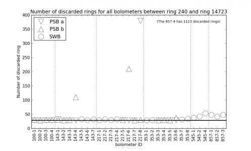
Fraction of discarded rings.
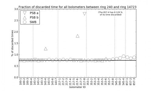
Fraction of time due to discarded rings.


Effective integration time[edit]
The following figure summarizes the effective integration time per bolometer. For that purpose the number of unflagged samples in non-discarded pointing periods have been used within the nominal mission. The average value is about 335 days of effective integration time.

Flag description[edit]
Input flags[edit]
The following flags are used as inputs to the TOI processing.
- The point-source flag (PSflag) -
- An earlier version of HFI point-source catalogue is read back in to flag TOIs, at a given frequency. In practice, 5σ sources are masked within a radius of 1.3 FWHM (which is 9, 7, 5, 5, 5, 5 arcmin at 100, 143, 217, 353, 545, and 857 GHz).
- The Galactic flag (Galflag) -
- An earlier version of HFI maps is thresholded and apodized. The produced masks are read into flag TOIs. The retained threshold corresponds to a sky coverage of, respectively, 70, 70, 80, 90, 90, and 90% at 100, 143, 217, 353, 545, and 857GHz.
- Solar System Object flag -
- For the TOI flag, Mars, Jupiter, and Saturn are flagged up to a radius of NBeam= 2, 3, 3, 4, 4, and 4 times the fiducial SSO_FWHM, with SSO_FWHM= 9, 7, 5, 5, 5, and 5 arcmin at 100, 143, 217, 353, 545, and 857GHz, respectively.
- As an input to the planet mask for maps, Mars, Jupiter, and Saturn are flagged with a radius computed as a coefficient depending on the planet (Factor_per_source) times NBeam times SSO_FWHM, with Factor_per_source = 1.1, 2.25, and 1.25 for Mars, Jupiter, and Saturn, respectively, and NBeam = 2.25, 4.25, 4.0, 5.0, 6.0, and 8.0 at 100, 143, 217, 353, 545, and 857GHz. This flag is called SSOflag4map.
- A small trailing tail is added to the mask to take into account the non-deconvolution of the planet signal, which has been replaced by background values. The width of this tail is 10% of the main flag diameter. The number of samples which are additionally flagged are Factor_per_Source times AddSNafter with "trail" × (Factor_per_source)3 samples, where trail = 10, 30, 20, 20, 30, and 40 at 100, 143, 217, 353, 545, and 857GHz, respectively.
- Uranus and Neptune, together with detected asteroids, are masked by HFI. They are masked at the TOI level using an exclusion radius of 1.5 times SSO_FWHM. At 857GHz, 24 asteroids have been detected with HFI, namely 1Ceres, 2Pallas, 3Juno, 4Vesta, 7Iris, 8Flora, 9Metis, 10Hygiea, 11Parthenope, 12Victoria, 13Egeria, 14Irene, 15Eunomia, 16Psyche, 18Melpomene, 19Fortuna, 20Massalia, 29Amphitrite, 41Daphne, 45Eugenia, 52Europa, 88Thisbe, 704Interamnia, and 324Bamberga.
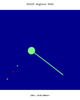
143 SWB row, around Jupiter first crossing.
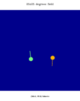
143 SWB row, around Saturn.
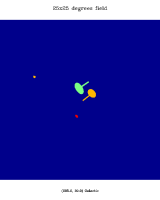
143 SWB row, around Mars.
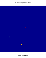
143 SWB row, random field in the ecliptic plane.
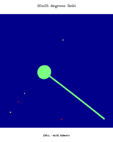
545/857 row, around Jupiter first crossing.
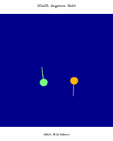
545/857 row, around Saturn.
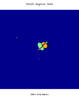
545/857 row, around Mars.
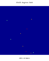
545/857 row, random field in the ecliptic plane.


Local maps showing the SSO flag. The colours correspond to the surveys involved in the nominal mission (green for Survey I, yellow for Survey 2, and red for Survey 3).
Output flags[edit]
A FlagTOIproc is produced by the TOI processing. It marks measurements which are not reliable for any of the following reasons.
- Gap (no valid input data), enlarged by one sample on each side. This flags less than 0.00044% (respectively 0.00062%) of the nominal (respectively complete) mission. It is equivalent to less than 3 (respectively 8) minutes of data.
- "Glitch" on dark bolometers: as the thermal template used for decorrelation is computed from these bolometer data, chunks of 1 minute-length data are discarded for all bolometers if at least 50% of the data for at least one dark bolometer are flagged during this time. This is efficient for flagging the data around the maximum of thermal events.
- "Glitch" on individual bolometers: samples where the signal from a cosmic ray hit dominates the sky signal at more than 3σ are discarded.
- Jump with 100 samples flagged around the computed position of the jump, to take into account the error on this reconstructed position.
The flag produced for the map making, called Total_flag, is therefore defined by
- Total_flag = UnstablePointing Flag OR FlagTOIproc OR SSOflag4map OR SSOflag, seen,
where FlagTOIproc = gap OR flag thermal template OR glitch OR jump and for PSB bolometers, FlagTOIproc_AB = FlagTOIproc_A OR FlagTOIproc_B. Note that the Total_flag is then identical for the A and B bolometers of a PSB pair.
At the destriping stage, a more restricted flag, called Total_flag_PS, is used. It is defined by Total_flag_PS = Total_flag OR PS_flag.
References[edit]
- ↑ Jump up to: 1.01.1 Planck 2013 results. VI. High Frequency Instrument Data Processing, Planck Collaboration, 2014, A&A, 571, A6.
- ↑ Jump up to: 2.02.1 Planck 2015 results. VII. High Frequency Instrument data processing: Time-ordered information and beam processing, Planck Collaboration, 2016, A&A, 594, A7.
- ↑ Jump up to: 3.03.1 Planck 2018 results. III. High Frequency Instrument data processing and frequency maps, Planck Collaboration, 2020, A&A, 641, A3.
- Jump up ↑ Planck 2013 results. X. HFI energetic particle effects: characterization, removal, and simulation, Planck Collaboration, 2014, A&A, 571, A10.
(Planck) High Frequency Instrument
analog to digital converter
(Planck) Low Frequency Instrument
Solar System Object
random telegraphic signal
Calibration and Performance Verification
sudden change of the baseline level inside a ring
Full-Width-at-Half-Maximum