Overview
This section describes the maps of astrophysical components produced from the Planck data. These products are derived from some or all of the nine frequency channel maps described above using different techniques and, in some cases, using other constraints from external data sets. Here we give a brief description of the product and how it is obtained, followed by a description of the FITS file containing the data and associated information.
All the details can be found in Planck-2013-XII[9].
CMB maps
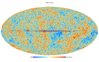
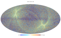
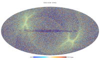
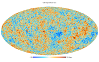
CMB maps have been produced by the SMICA, NILC, SEVEM and COMMANDER-Ruler pipelines. Of these, the SMICA product is considered the preferred one overall and is labelled Main product in the Planck Legacy Archive, while the other two are labeled as Additional product.
SMICA and NILC also produce inpainted maps, in which the Galactic Plane, some bright regions and masked point sources are replaced with a constrained CMB realization such that the whole map has the same statistical distribution as the observed CMB.
The results of SMICA, NILC and SEVEM pipeline are distributed as a FITS file containing 4 extensions:
- CMB maps and ancillary products (3 or 6 maps)
- CMB-cleaned foreground maps from LFI (3 maps)
- CMB-cleaned foreground maps from HFI (6 maps)
- Effective beam of the CMB maps (1 vector)
The results of COMMANDER-Ruler are distributed as two FITS files (the high and low resolution) containing the following extensions:
High resolution N$_\rm{side}$=2048 (note that we don't provide the CMB-cleaned foregrounds maps for LFI and HFI because the Ruler resolution (~7.4') is lower than the HFI highest channel and and downgrading it will introduce noise correlation).
- CMB maps and ancillary products (4 maps)
- Effective beam of the CMB maps (1 vector)
Low resolution N$_\rm{side}$=256
- CMB maps and ancillary products (3 maps)
- 10 example CMB maps used in the montecarlo realization (10 maps)
- Effective beam of the CMB maps (1 vector)
For a complete description of the data structure, see the below; the content of the first extensions is illustrated and commented in the table below.
The maps (CMB, noise, masks) contained in the first extension
| Col name
|
SMICA
|
NILC
|
SEVEM
|
COMMANDER-Ruler H
|
COMMANDER-Ruler L
|
Description / notes
|
|---|
| 1: I
|

|

|
|
|
|
Raw CMB anisotropy map. These are the maps used in the component separation paper Planck-2013-XII[9].
|
| 2: NOISE
|
|
|
|
|
not applicable
|
Noise map. Obtained by propagating the half-ring noise through the CMB cleaning pipelines.
|
| 3: VALMASK
|
|
|
|
|
|
Confidence map. Pixels with an expected low level of foreground contamination. These maps are only indicative and obtained by different ad hoc methods. They cannot be used to rank the CMB maps.
|
| 4: I_MASK
|
|
|
not applicable
|
not applicable
|
not applicable
|
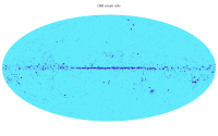
Some areas are masked for the production of the raw CMB maps (for NILC: point sources from 44 GHz to 857 GHz; for SMICA: point sources from 30 GHz to 857 GHz, Galatic region and additional bright regions).
|
| 5: INP_CMB
|

|
|
not applicable
|
not applicable
|
not applicable
|
Inpainted CMB map. The raw CMB maps with some regions (as indicated by INP_MASK) replaced by a constrained Gaussian realization. The inpainted SMICA map was used for PR.
|
| 6: INP_MASK
|
|
|
not applicable
|
not applicable
|
not applicable
|
Mask of the inpainted regions. For SMICA, this is identical to I_MASK. For NILC, it is not.
|
The component separation pipelines are described in the CMB and foreground separation section and also in Section 3 and Appendices A-D of Planck-2013-XII[9] and references therein.
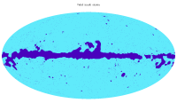
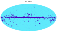
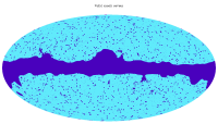
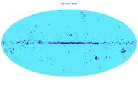
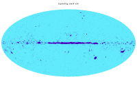
The union (or common) mask is defined as the union of the confidence masks from the four component separation pipelines, the three listed above and Commander-Ruler. It leaves 73% of the sky available, and so it is denoted as U73.
Product description
SMICA
- Principle
- SMICA produces a CMB map by linearly combining all Planck input channels (from 30 to 857 GHz) with weights which vary with the multipole. It includes multipoles up to \ell = 4000.
- Resolution (effective beam)
- The SMICA map has an effective beam window function of 5 arc-minutes truncated at \ell=4000 and deconvolved from the pixel window. It means that, ideally, one would have C_\ell(map) = C_\ell(sky) * B_\ell(5')^2, where C_\ell(map) is the angular spectrum of the map, where C_\ell(sky) is the angular spectrum of the CMB and B_\ell(5') is a 5-arcminute Gaussian beam function. Note however that, by convention, the effective beam window function B_\ell(fits) provided in the FITS file does include a pixel window function. Therefore, it is equal to B_\ell(fits) = B_\ell(5') / p_\ell(2048) where p_\ell(2048) denotes the pixel window function for an Nside=2048 pixelization.
- Confidence mask
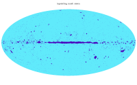
- A confidence mask is provided which excludes some parts of the Galactic plane, some very bright areas and the masked point sources. This mask provides a qualitative (and subjective) indication of the cleanliness of a pixel.
- Masks and inpainting
- The raw SMICA CMB map has valid pixels except at the location of masked areas: point sources, Galactic plane, some other bright regions. Those invalid pixels are indicated with the mask named 'I_MASK'. The raw SMICA map has been inpainted, producing the map named "INP_CMB". Inpainting consists in replacing some pixels (as indicated by the mask named INP_MASK) by the values of a constrained Gaussian realization which is computed to ensure good statistical properties of the whole map (technically, the inpainted pixels are a sample realisation drawn under the posterior distribution given the un-masked pixels.
NILC
- Principle
- The Needlet-ILC (hereafter NILC) CMB map is constructed from all Planck channels from 44 to 857 GHz and includes multipoles up to \ell = 3200. It is obtained by applying the Internal Linear Combination (ILC) technique in needlet space, that is, with combination weights which are allowed to vary over the sky and over the whole multipole range.
- Resolution (effective beam)
- As in the SMICA product except that there is no abrupt truncation at \ell_{max}= 3200 but a smooth transition to 0 over the range 2700\leq\ell\leq 3200.
- Confidence mask
- A confidence mask is provided which excludes some parts of the Galactic plane, some very bright areas and the masked point sources. This mask provides a qualitative indication of the cleanliness of a pixel. The threshold is somewhat arbitrary.
- Masks and inpainting
- The raw NILC map has valid pixels except at the location of masked point sources. This is indicated with the mask named 'I_MASK'. The raw NILC map has been inpainted, producing the map named "INP_CMB". The inpainting consists in replacing some pixels (as indicated by the mask named INP_MASK) by the values of a constrained Gaussian realization which is computed to ensure good statistical properties of the whole map (technically, the inpainted pixels are a sample realisation drawn under the posterior distribution given the un-masked pixels.
SEVEM
The aim of SEVEM is to produce clean CMB maps at one or several frequencies by using a procedure based on template fitting. The templates are internal, i.e., they are constructed from Planck data, avoiding the need for external data sets, which usually complicates the analyses and may introduce inconsistencies. The method has been successfully applied to Planck simulations[10] and to WMAP polarisation data[11]. In the cleaning process, no assumptions about the foregrounds or noise levels are needed, rendering the technique very robust. Note that unlike the other products, SEVEM does not provide the mask of regions not used in the productions of the CMB ma (I_MASK) nor an inpainted version of the map and its associated mask. On the other hand, it provides channel maps and 100, 143, and 217 GHz which are used as the building blocks of the final map.
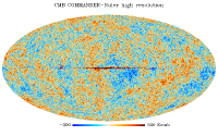
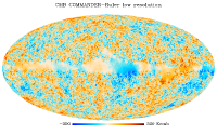
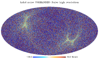
COMMANDER-Ruler
COMMANDER-Ruler is the Planck software implementing a pixel based parametric component separation. Amplitude of CMB and the main diffuse foregrounds along with the relevant spectral parameters for those (see below in the Astrophysical Foreground Section for the latter) are parametrized and fitted in single MCMC chains conducted at $N_\rm{side}$=256 using COMMANDER, implementing a Gibbs Sampling. The CMB amplitude which
is obtained in these runs corresponds to the delivered low resolution CMB component from COMMANDER-Ruler which has a FWHM of 40 arcminutes. The sampling of the foreground parameters is applied to the data at full resolution for obtaining the high resolution CMB component from Ruler which is available on the PLA. In the Planck Component Separation paper[9] additional material is discussed, specifically concerning the sky region where the solutions are reliable, in terms of chi2 maps. The products mainly consist of:
- Maps of the Amplitudes of the CMB at low resolution, $N_\rm{side}$=256, along with the standard deviations of the outputs, beam profiles derived from the production process.
- Maps of the CMB amplitude, along with the standard deviations, at high resolution, $N_\rm{side}$=2048, beam profiles derived from the production process.
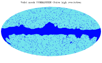
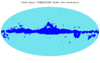
- Mask obtained on the basis of the precision in the fitting procedure; the thresholding is evaluated through the COMMANDER-Ruler likelihood analysis and excludes 13% of the sky, see Planck-2013-XII[9].
Production process
SMICA
- 1) Pre-processing
- All input maps undergo a pre-processing step to deal with point sources. The point sources with SNR > 5 in the PCCS catalogue are fitted in each input map. If the fit is successful, the fitted point source is removed from the map; otherwise it is masked and the hole is filled in by a simple diffusive process to ensure a smooth transition and mitigate spectral leakage. This is done at all frequencies but 545 and 857 GHz, here all point sources with SNR > 7.5 are masked and filled-in similarly.
- 2) Linear combination
- The nine pre-processed Planck frequency channels from 30 to 857 GHzare harmonically transformed up to \ell = 4000 and co-added with multipole-dependent weights as shown in the figure.
- 3) Post-processing
- The areas masked in the pre-processing step are replaced by a constrained Gaussian realization.
Note: The visible power deficit in the raw CMB map around the galactic plane is due to the smooth fill-in of the masked areas in the input maps (the result of the pre-processing). It is not to be confused with the post-processing step of inpainting of the CMB map with a constrained Gaussian realization.
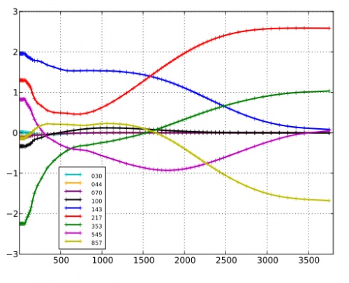
Weights given by SMICA to the input maps (after they are re-beamed to 5 arcmin and expressed in K_\rm{RJ}), as a function of multipole. NILC
- 1) Pre-processing
- Same pre-processing as SMICA (except the 30 GHz channel is not used).
- 2) Linear combination
- The pre-processed Planck frequency channels from 44 to 857 GHz are linearly combined with weights which depend on location on the sky and on the multipole range up to \ell = 3200. This is achieved using a needlet (redundant spherical wavelet) decomposition. For more details, see Planck-2013-XII[9].
- 3) Post-processing
- The areas masked in the pre-processing plus other bright regions step are replaced by a constrained Gaussian realization as in the SMICA post-processing step.
SEVEM
The templates are internal, i.e., they are constructed from Planck data, avoiding the need for external data sets, which usually complicates the analyses and may introduce inconsistencies. In the cleaning process, no assumptions about the foregrounds or noise levels are needed, rendering the technique very robust. The fitting can be done in real or wavelet space (using a fast wavelet adapted to the HEALPix pixelization[12]) to properly deal with incomplete sky coverage. By expediency, however, we fill in the small number of unobserved pixels at each channel with the mean value of its neighbouring pixels before applying SEVEM.
We construct our templates by subtracting two close Planck frequency channel maps, after first smoothing them to a common resolution to ensure that the CMB signal is properly removed. A linear combination of the templates t_j is then subtracted from (hitherto unused) map d to produce a clean CMB map at that frequency. This is done either in real or in wavelet space (i.e., scale by scale) at each position on the sky: T_c(\mathbf{x}, ν) = d(\mathbf{x}, ν) − \sum_{j=1}^{n_t} α_j t(\mathbf{x})
where n_t is the number of templates. If the cleaning is performed in real space, the α_j coefficients are obtained by minimising the variance of the clean map T_c outside a given mask. When working in wavelet space, the cleaning is done in the same way at each wavelet scale independently (i.e., the linear coefficients depend on the scale). Although we exclude very contaminated regions during the minimization, the subtraction is performed for all pixels and, therefore, the cleaned maps cover the full-sky (although we expect that foreground residuals are present in the excluded areas).
An additional level of flexibility can also be considered: the linear coefficients can be the same for all the sky, or several regions with different sets of coefficients can be considered. The regions are then combined in a smooth way, by weighting the pixels at the boundaries, to avoid discontinuities in the clean maps.
Since the method is linear, we may easily propagate the noise properties to the final CMB map. Moreover, it is very fast and permits the generation of thousands of simulations to character- ize the statistical properties of the outputs, a critical need for many cosmological applications. The final CMB map retains the angular resolution of the original frequency map.
There are several possible configurations of SEVEM with regard to the number of frequency maps which are cleaned or the number of templates that are used in the fitting. Note that the production of clean maps at different frequencies is of great interest in order to test the robustness of the results. Therefore, to define the best strategy, one needs to find a compromise between the number of maps that can be cleaned independently and the number of templates that can be constructed.
In particular, we have cleaned the 143 GHz and 217 GHz maps using four templates constructed as the difference of the following Planck channels (smoothed to a common resolution): (30-44), (44-70), (545-353) and (857-545). For simplicity, the three maps have been cleaned in real space, since there was not a significant improvement when using wavelets (especially at high latitude). In order to take into account the different spectral behaviour of the foregrounds at low and high galactic latitudes, we have considered two independent regions of the sky, for which we have used a different set of coefficients. The first region corresponds to the 3 per cent brightest Galactic emission, whereas the second region is defined by the remaining 97 per cent of the sky. For the first region, the coefficients are actually estimated over the whole sky (we find that this is more optimal than perform the minimisation only on the 3 per cent brightest region, where the CMB emission is very sub-dominant) while for the second region, we exclude the 3 per cent brightest region of the sky, point sources detected at any frequency and those pixels which have not been observed at all channels.
Our final CMB map has then been constructed by combining the 143 and 217 GHz maps by weighting the maps in harmonic space taking into account the noise level, the resolution and a rough estimation of the foreground residuals of each map (obtained from realistic simulations). This final map has a resolution corresponding to a Gaussian beam of fwhm=5 arcminutes.
Moreover, additional CMB clean maps (at frequencies between 44 and 353 GHz) have also been produced using different combinations of templates for some of the analyses carried out in Planck-2013-XXIII[13] and Planck-2013-XIX[14]. In particular, clean maps from 44 to 353 GHz have been used for the stacking analysis presented in Planck-2013-XIX[14], while frequencies from 70 to 217 GHz were used for consistency tests in Planck-2013-XXIII[13].
COMMANDER-Ruler
The production process consist in low and high resolution runs according to the description above.
- Low Resolution Runs
- Same as the Astrophysics Foregrounds Section below; The CMB amplitude is fitted along with the other foreground parameters and constitutes the CMB Low Resolution Rendering which is in the PLA.
- Ruler Runs
- the sampling at high resolution is used to infer the probability distribution of spectral parameters which is exploited at full resolution in order to obtain the High Resolution CMB Rendering which is in the PLA.
Masks
Summary table with the different masks that have been used by the component separation methods to pre-process and to process the frequency maps and the CMB maps.
| Commander 2013 (PR1) |
Used for diffuse inpainting of input frequency maps |
Used for constrained Gaussian realization inpaiting of CMB map |
Description
|
|---|
| VALMASK |
NO |
NO |
VALMASK is the confidence mask that defines the region where the reconstructed CMB is trusted. It can be found inside
COM_CompMap_CMB-commrul_2048_R1.00.fits and COM_CompMap_CMB-commrul_0256_R1.00.fits for low resolution analyses.
|
|
|
|
|
|
|---|
| SEVEM 2013 (PR1) |
Used diffuse inpainting of input frequency maps |
Used for Constrained Gaussian realization inpaiting of CMB map |
Description
|
|---|
| VALMASK |
NO |
NO |
VALMASK is the confidence mask that defines the region where the reconstructed CMB is trusted. It can be found inside
COM_CompMap_CMB-sevem_2048_R1.12.fits.
|
|
|
|
|
|
|---|
| NILC 2013 (PR1) |
Used for diffuse inpainting of input frequency maps |
Used for constrained Gaussian realization inpaiting of CMB map |
Description
|
|---|
| VALMASK |
NO |
NO |
VALMASK is the confidence mask that defines the region where the reconstructed CMB is trusted. It can be found inside COM_CompMap_CMB-nilc_2048_R1.20.fits.
|
| I_MASK |
NO |
NO |
I_MASK defines the regions over which CMB is not built. It is a combination of point source masks, Galactic plane mask and other bright regions like LMC, SMC, etc. It can be found inside COM_CompMap_CMB-nilc_2048_R1.20.fits.
|
| INP_MASK |
NO |
YES |
It can be found inside COM_CompMap_CMB-nilc_2048_R1.20.fits.
|
|
|
|
|
|
|---|
| SMICA 2013 (PR1) |
Used for diffuse inpainting of input frequency maps |
Used for constrained Gaussian realization inpaiting of CMB map |
Description
|
|---|
| VALMASK |
NO |
NO |
VALMASK is the confidence mask that defines the region where the reconstructed CMB is trusted. It can be found inside
COM_CompMap_CMB-smica_2048_R1.20.fits.
|
| I_MASK |
YES |
YES |
I_MASK defines the regions over which CMB is not built. It is a combination of point source masks, Galactic plane mask and other bright regions like LMC, SMC, etc. It can be found inside COM_CompMap_CMB-smica_2048_R1.20.fits.
|
| INP_MASK |
YES |
YES |
INP_MASK for SMICA 2013 release is identical to I_MASK above.
|
Inputs
The input maps are the sky temperature maps described in the Sky temperature maps section. SMICA and SEVEM use all the maps between 30 and 857 GHz; NILC uses the ones between 44 and 857 GHz. Commander-Ruler uses frequency channel maps from 30 to 353 GHz.
File names and structure
The FITS files corresponding to the three CMB products are the following:
The files contain a minimal primary extension with no data and four BINTABLE data extensions. Each column of the BINTABLE is a (Healpix) map; the column names and the most important keywords of each extension are described in the table below; for the remaining keywords, please see the FITS files directly.
CMB map file data structure
| Ext. 1. EXTNAME = COMP-MAP (BINTABLE)
|
|---|
| Column Name |
Data Type |
Units |
Description
|
|---|
| I |
Real*4 |
uK_cmb |
CMB temperature map
|
| NOISE |
Real*4 |
uK_cmb |
Estimated noise map (note 1)
|
| I_STDEV |
Real*4 |
uK_cmb |
Standard deviation, ONLY on COMMANDER-Ruler products
|
| VALMASK |
Byte |
none |
Confidence mask (note 2)
|
| I_MASK |
Byte |
none |
Mask of regions over which CMB map is not built (Optional - see note 3)
|
| INP_CMB |
Real*4 |
uK_cmb |
Inpainted CMB temperature map (Optional - see note 3)
|
| INP_MASK |
Byte |
none |
mask of inpainted pixels (Optional - see note 3)
|
| Keyword |
Data Type |
Value |
Description
|
|---|
| AST-COMP |
String |
CMB |
Astrophysical compoment name
|
| PIXTYPE |
String |
HEALPIX |
|
| COORDSYS |
String |
GALACTIC |
Coordinate system
|
| ORDERING |
String |
NESTED |
Healpix ordering
|
| NSIDE |
Int |
2048 |
Healpix Nside
|
| METHOD |
String |
name |
Cleaning method (SMICA/NILC/SEVEM/COMMANDER-Ruler)
|
| Ext. 2. EXTNAME = FGDS-LFI (BINTABLE) - Note 4
|
|---|
| Column Name |
Data Type |
Units |
Description
|
|---|
| LFI_030 |
Real*4 |
K_cmb |
30 GHz foregrounds
|
| LFI_044 |
Real*4 |
K_cmb |
44 GHz foregrounds
|
| LFI_070 |
Real*4 |
K_cmb |
70 GHz foregrounds
|
| Keyword |
Data Type |
Value |
Description
|
|---|
| PIXTYPE |
String |
HEALPIX |
|
| COORDSYS |
String |
GALACTIC |
Coordinate system
|
| ORDERING |
String |
NESTED |
Healpix ordering
|
| NSIDE |
Int |
1024 |
Healpix Nside
|
| METHOD |
String |
name |
Cleaning method (SMICA/NILC/SEVEM)
|
| Ext. 3. EXTNAME = FGDS-HFI (BINTABLE) - Note 4
|
|---|
| Column Name |
Data Type |
Units |
Description
|
|---|
| HFI_100 |
Real*4 |
K_cmb |
100 GHz foregrounds
|
| HFI_143 |
Real*4 |
K_cmb |
143 GHz foregrounds
|
| HFI_217 |
Real*4 |
K_cmb |
217 GHz foregrounds
|
| HFI_353 |
Real*4 |
K_cmb |
353 GHz foregrounds
|
| HFI_545 |
Real*4 |
MJy/sr |
545 GHz foregrounds
|
| HFI_857 |
Real*4 |
MJy/sr |
857 GHz foregrounds
|
| Keyword |
Data Type |
Value |
Description
|
|---|
| PIXTYPE |
String |
HEALPIX |
|
| COORDSYS |
String |
GALACTIC |
Coordinate system
|
| ORDERING |
String |
NESTED |
Healpix ordering
|
| NSIDE |
Int |
2048 |
Healpix Nside
|
| METHOD |
String |
name |
Cleaning method (SMICA/NILC/SEVEM/COMMANDER-Ruler)
|
| Ext. 4. EXTNAME = BEAM_WF (BINTABLE)
|
|---|
| Column Name |
Data Type |
Units |
Description
|
|---|
| BEAM_WF |
Real*4 |
none |
The effective beam window function, including the pixel window function. See Note 5.
|
| Keyword |
Data Type |
Value |
Description
|
|---|
| LMIN |
Int |
value |
First multipole of beam WF
|
| LMAX |
Int |
value |
Lsst multipole of beam WF
|
| METHOD |
String |
name |
Cleaning method (SMICA/NILC/SEVEM/COMMANDER-Ruler)
|
Notes:
- The half-ring half-difference (HRHD) map is made by passing the half-ring frequency maps independently through the component separation pipeline, then computing half their difference. It approximates a noise realisation, and gives an indication of the uncertainties due to instrumental noise in the corresponding CMB map.
- The confidence mask indicates where the CMB map is considered valid.
- This column is not present in the SEVEM and COMMANDER-Ruler product file. For SEVEM these three columns give the CMB channel maps at 100, 143, and 217 GHz (columns C100, C143, and C217, in units of K_cmb.
- The subtraction of the CMB from the sky maps in order to produce the foregrounds map is done after convolving the CMB map to the resolution of the given frequency. Those columns are not present in the COMMANDER-Ruler product file.
- The beam window function B_\ell given here includes the pixel window function p_\ell for the Nside=2048 pixelization. It means that, ideally, C_\ell(map) = C_\ell(sky) \, B_\ell^2 \, p_\ell^2.
The low resolution COMMANDER-Ruler CMB product is organized in the following way:
CMB low resolution COMMANDER-Ruler map file data structure
| Ext. 1. EXTNAME = COMP-MAP (BINTABLE)
|
|---|
| Column Name |
Data Type |
Units |
Description
|
|---|
| I |
Real*4 |
uK_cmb |
CMB temperature map obtained as average over 1000 samples
|
| I_stdev |
Real*4 |
uK_cmb |
Corresponding Standard deviation amongst the 1000 samples
|
| VALMASK |
Byte |
none |
Confidence mask
|
| Keyword |
Data Type |
Value |
Description
|
|---|
| PIXTYPE |
String |
HEALPIX |
|
| COORDSYS |
String |
GALACTIC |
Coordinate system
|
| ORDERING |
String |
NESTED |
Healpix ordering
|
| NSIDE |
Int |
2048 |
Healpix Nside
|
| METHOD |
String |
name |
Cleaning method (SMICA/NILC/SEVEM/COMMANDER-Ruler)
|
| Ext. 2. EXTNAME = CMB-Sample (BINTABLE)
|
|---|
| Column Name |
Data Type |
Units |
Description
|
|---|
| I_SIM01 |
Real*4 |
K_cmb |
CMB Sample, smoothed to 40 arcmin
|
| I_SIM02 |
Real*4 |
K_cmb |
CMB Sample, smoothed to 40 arcmin
|
| I_SIM03 |
Real*4 |
K_cmb |
CMB Sample, smoothed to 40 arcmin
|
| I_SIM04 |
Real*4 |
K_cmb |
CMB Sample, smoothed to 40 arcmin
|
| I_SIM05 |
Real*4 |
K_cmb |
CMB Sample, smoothed to 40 arcmin
|
| I_SIM06 |
Real*4 |
K_cmb |
CMB Sample, smoothed to 40 arcmin
|
| I_SIM07 |
Real*4 |
K_cmb |
CMB Sample, smoothed to 40 arcmin
|
| I_SIM08 |
Real*4 |
K_cmb |
CMB Sample, smoothed to 40 arcmin
|
| I_SIM09 |
Real*4 |
K_cmb |
CMB Sample, smoothed to 40 arcmin
|
| I_SIM10 |
Real*4 |
K_cmb |
CMB Sample, smoothed to 40 arcmin
|
| Keyword |
Data Type |
Value |
Description
|
|---|
| PIXTYPE |
String |
HEALPIX |
|
| COORDSYS |
String |
GALACTIC |
Coordinate system
|
| ORDERING |
String |
NESTED |
Healpix ordering
|
| NSIDE |
Int |
1024 |
Healpix Nside
|
| METHOD |
String |
name |
Cleaning method (SMICA/NILC/SEVEM/COMMANDER-Ruler)
|
| Ext. 4. EXTNAME = BEAM_WF (BINTABLE)
|
|---|
| Column Name |
Data Type |
Units |
Description
|
|---|
| BEAM_WF |
Real*4 |
none |
The effective beam window function, including the pixel window function.
|
| Keyword |
Data Type |
Value |
Description
|
|---|
| LMIN |
Int |
value |
First multipole of beam WF
|
| LMAX |
Int |
value |
Lsst multipole of beam WF
|
| METHOD |
String |
name |
Cleaning method (SMICA/NILC/SEVEM/COMMANDER-Ruler)
|
The FITS files containing the union (or common) maks is:
which contains a single BINTABLE extension with a single column (named U73) for the mask, which is boolean (FITS TFORM = B), in GALACTIC coordinates, NESTED ordering, and Nside=2048.
For the benefit of users who are only looking for a small file containing the SMICA cmb map with no additional information (noise or masks) we provide such a file here
This file contains a single extension with a single column containing the SMICA cmb temperature map.
Cautionary notes
- The half-ring CMB maps are produced by the pipelines with parameters/weights fixed to the values obtained from the full maps. Therefore the CMB HRHD maps do not capture all of the uncertainties due to foreground modelling on large angular scales.
- The HRHD maps for the HFI frequency channels underestimate the noise power spectrum at high l by typically a few percent. This is caused by correlations induced in the pre-processing to remove cosmic ray hits. The CMB is mostly constrained by the HFI channels at high l, and so the CMB HRHD maps will inherit this deficiency in power.
- The beam transfer functions do not account for uncertainties in the beams of the frequency channel maps.
Astrophysical foregrounds from parametric component separation
We describe diffuse foreground products for the Planck 2013 release. See Planck Component Separation paper Planck-2013-XII[9] for a detailed description and astrophysical discussion of those.
Product description
- Low frequency foreground component
- The products below contain the result of the fitting for one foreground component at low frequencies in Planck bands,along with its spectral behavior parametrized by a power law spectral index. Amplitude and spectral indeces are evaluated at N$_\rm{side}$ 256 (see below in the production process), along with standard deviation from sampling and instrumental noise on both. An amplitude solution at N$_\rm{side}$=2048 is also given, along with standard deviation from sampling and instrumental noise as well as solutions on halfrings. The beam profile associated to this component is also provided as a secondary Extension in the N$_\rm{side}$ 2048 product.
- Thermal dust
- The products below contain the result of the fitting for one foreground component at high frequencies in Planck bands, along with its spectral behavior parametrized by temperature and emissivity. Amplitude, temperature and emissivity are evaluated at N$_\rm{side}$ 256 (see below in the production process), along with standard deviation from sampling and instrumental noise on all of them. An amplitude solution at N$_\rm{side}$=2048 is also given, along with standard deviation from sampling and instrumental noise as well as solutions on halfrings. The beam profile associated to this component is provided.
- Sky mask
- The delivered mask is defined as the sky region where the fitting procedure was conducted and the solutions presented here were obtained. It is made by masking a region where the Galactic emission is too intense to perform the fitting, plus the masking of brightest point sources.
Production process
CODE: COMMANDER-RULER. The code exploits a parametrization of CMB and main diffuse foreground observables. The naive resolution of input
frequency channels is reduced to N$_\rm{side}$=256 first. Parameters related to the foreground scaling with frequency are estimated at that resolution
by using Markov Chain Monte Carlo analysis using Gibbs sampling. The foreground parameters make the foreground mixing matrix which is
applied to the data at full resolution in order to obtain the provided products at N$_\rm{side}$=2048. In the Planck Component Separation paper Planck-2013-XII[9] additional material is discussed, specifically concerning the sky region where the solutions are reliable, in terms of chi2 maps.
Inputs
Nominal frequency maps at 30, 44, 70, 100, 143, 217, 353 GHz (LFI 30 GHz frequency maps, LFI 44 GHz frequency maps and LFI 70 GHz frequency maps, HFI 100 GHz frequency maps, HFI 143 GHz frequency maps,HFI 217 GHz frequency maps and HFI 353 GHz frequency maps) and their II column corresponding to the noise covariance matrix.
Halfrings at the same frequencies. Beam window functions as reported in the LFI and HFI RIMO.
Related products
None.
File names
Meta Data
Low frequency foreground component
Low frequency component at N$_\rm{side}$ = 256
File name: COM_CompMap_Lfreqfor-commrul_0256_R1.00.fits
- Name HDU -- COMP-MAP
The Fits extension is composed by the columns described below:
FITS header
| Column Name |
Data Type |
Units |
Description
|
|---|
| I |
Real*4 |
uK[math]_{CMB}[/math] |
Intensity
|
| I_stdev |
Real*4 |
uK[math]_{CMB}[/math] |
standard deviation of intensity
|
| Beta |
Real*4 |
|
effective spectral index
|
| B_stdev |
Real*4 |
|
standard deviation on the effective spectral index
|
- Notes
- Comment: The Intensity is normalized at 30 GHz
- Comment: The intensity was estimated during mixing matrix estimation
Low frequency component at N$_\rm{side}$ = 2048
- File name: COM_CompMap_Lfreqfor-commrul_2048_R1.00.fits
- Name HDU -- COMP-MAP
The Fits extension is composed by the columns described below:
FITS header
| Column Name |
Data Type |
Units |
Description
|
|---|
| I |
Real*8 |
uK[math]_{CMB}[/math] |
Intensity
|
| I_stdev |
Real*8 |
uK[math]_{CMB}[/math] |
standard deviation of intensity
|
| I_hr1 |
Real*8 |
uK[math]_{CMB}[/math] |
Intensity on half ring 1
|
| I_hr2 |
Real*8 |
uK[math]_{CMB}[/math] |
Intensity on half ring 2
|
- Notes
- Comment: The intensity was computed after mixing matrix application
- Name HDU -- BeamWF
The Fits second extension is composed by the columns described below:
FITS header
| Column Name |
Data Type |
Units |
Description
|
|---|
| BeamWF |
Real*4 |
|
beam profile
|
- Notes
- Comment: Beam window function used in the Component separation process
Thermal dust
Thermal dust component at N$_\rm{side}$=256
- File name: COM_CompMap_dust-commrul_0256_R1.00.fits
- Name HDU -- COMP-MAP
The Fits extension is composed by the columns described below:
FITS header
| Column Name |
Data Type |
Units |
Description
|
|---|
| I |
Real*4 |
MJy/sr |
Intensity
|
| I_stdev |
Real*4 |
MJy/sr |
standard deviation of intensity
|
| Em |
Real*4 |
|
emissivity
|
| Em_stdev |
Real*4 |
|
standard deviation on emissivity
|
| T |
Real*4 |
uK[math]_{CMB}[/math] |
temperature
|
| T_stdev |
Real*4 |
uK[math]_{CMB}[/math] |
standard deviation on temerature
|
- Notes
- Comment: The intensity is normalized at 353 GHz
Thermal dust component at N$_\rm{side}$=2048
File name: COM_CompMap_dust-commrul_2048_R1.00.fits
- Name HDU -- COMP-MAP
The Fits extension is composed by the columns described below:
FITS header
| Column Name |
Data Type |
Units |
Description
|
|---|
| I |
Real*8 |
MJy/sr |
Intensity
|
| I_stdev |
Real*8 |
MJy/sr |
standard deviation of intensity
|
| I_hr1 |
Real*8 |
MJy/sr |
Intensity on half ring 1
|
| I_hr2 |
Real*8 |
MJy/sr |
Intensity on half ring 2
|
- Name HDU -- BeamWF
The Fits second extension is composed by the columns described below:
FITS header
| Column Name |
Data Type |
Units |
Description
|
|---|
| BeamWF |
Real*4 |
|
beam profile
|
- Notes
- Comment: Beam window function used in the Component separation process
Sky mask
File name: COM_CompMap_Mask-rulerminimal_2048.fits
- Name HDU -- COMP-MASK
The Fits extension is composed by the columns described below:
FITS header
| Column Name |
Data Type |
Units |
Description
|
|---|
| Mask |
Real*4 |
|
Mask
|
Thermal dust emission
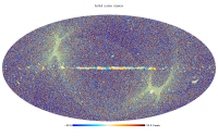
Thermal emission from interstellar dust is captured by Planck-HFI over the whole sky, at all frequencies from 100 to 857 GHz. This emission is well modelled by a modified black body in the far-infrared to millimeter range. It is produced by the biggest interstellar dust grain that are in thermal equilibrium with the radiation field from stars. The grains emission properties in the sub-millimeter are therefore directly linked to their absorption properties in the UV-visible range. By modelling the thermal dust emission in the sub-millimeter, a map of dust reddening in the visible can then be constructed. The details of the model can be found here Planck-2013-XI[15].
Model of all-sky thermal dust emission
The model of the thermal dust emission is based on a modified black body (MBB) fit to the data I_\nu
- I_\nu = A\, B_\nu(T)\, \nu^\beta
where B_\nu(T) is the Planck function for dust equilibirum temperature T, A is the amplitude of the MBB and \beta the dust spectral index. The dust optical depth at frequency \nu is
- \tau_\nu = I_\nu / B_\nu(T) = A\, \nu^\beta
The dust parameters provided are T, \beta and \tau_{353}. They were obtained by fitting the Planck data at 353, 545 and 857 GHz (from which the Planck zodiacal light model was removed) together with the IRAS 100 micron data. The latter is a combination of the 100 micron maps from IRIS (Miville-Deschenes & Lagache, 2005) and from Schlegel et al. (1998), SFD1998. The IRIS (SFD1998) map is used at scales smaller (larger) than 30 arcmin; this combination allows to take advantage of the higher angular resolution and better control of gain variations of the IRIS map and of the better removal of the zodiacal light emission of the SFD1998 map.
All maps (in Healpix Nside=2048 were smoothed to a common resolution of 5 arcmin. The CMB anisotropies, clearly visible at 353 GHz, were removed from all the HFI maps using the SMICA map. An offset was removed from each map to set a Galactic zero level, using a correlation with the LAB 21 cm data in diffuse areas of the sky (N_{HI} \lt 2\times10^{20} cm^{-2}). Because the dust emission is so well correlated between frequencies in the Rayleigh-Jeans part of the dust spectrum, the zero level of the 545 and 353 GHz were improved by correlating with the 857 GHz over a larger mask (N_{HI} \lt 3\times10^{20} cm^{-2}). Faint residual dipole structures, identified in the 353 and 545 GHz maps, were removed prior to the fit.
The MBB fit was performed using a \chi^2 minimization method, assuming errors for each data point that include instrumental noise, calibration uncertainties (on both the dust emission and the CMB anisotropies) and uncertainties on the zero levels. Because of the known degeneracy between T and \beta in the presence of noise, we performed tge fit in two steps. First we produced a model of dust emission using data smoothed to 30 arcmin; at such resolution no systematic bias of the parameters is observed. In a second step the map of the spectral index \beta at 30 arcmin was used to fit the data for T and \tau_{353} at 5 arcmin.
The E(B-V) map for extra-galactic studies
For the production of the E(B-V) map, we used a MBB fit to Planck and IRAS data from which point sources were removed to avoid contamination by galaxies. In the hypothesis of constant dust emission cross-section, the optical depth map \tau_{353} is proportional to dust column density and therefore often used to estimate E(B-V). The analysis of Planck data revealed that the ratio \tau_{353}/N_{HI} and \tau_{353}/E(B-V) are not constant, even in the diffuse ISM, but that they depend on T revealing possible spatial variations of the dust emission cross-section. It appears that the dust radiance, R, i.e. the dust emission integrated in frequency, is a better tracer of column density in the diffuse ISM, implying small spatial variations of the radiation field strength at high Galactic latitude.
Given those results, we also deliver the map of R as a dust product and we propose to use it as an estimator of Galactic dust reddening for extra-galactic studies: E(B-V) = q\, R.
To estimate the calibration factor q, we followed a method similar to[16] based on SDSS reddening measurements of quasars in the u, g, r, i and z bands[17]. We used a sample of 53 399 quasars, selecting objects at redshifts for which Ly\alpha does not enter the SDSS filters. The interstellar HI column densities covered on the lines of sight of this sample ranges from 0.5 to 10\times10^{20}\,cm^{-2}. Therefore this sample allows us to estimate q in the diffuse ISM where this map of E(B-V) is intended to be used.
Dust optical depth products
The dust model maps are found in the file HFI_CompMap_ThermalDustModel_2048_R1.20.fits (see the note below for an important clarification regarding the thermal dust model); its characteristics are:
- Dust optical depth at 353 GHz: Nside=2048, fwhm=5', no units
- Dust temperature: Nside 2048, fwhm=5', units=Kelvin
- Dust spectral index: Nside=2048, fwhm=30', no units
- Dust radiance: Nside=2048, fwhm=5', units=Wm-2sr-1
- E(B-V) for extragalactic studies: Nside=2048, fwhm=5', units=magnitude, obtained with data from which point sources were removed.
Dust opacity file data structure
| 1. EXTNAME = 'COMP-MAP'
|
|---|
| Column Name |
Data Type |
Units |
Description
|
|---|
| TAU353 |
Real*4 |
none |
The optical depth at 353GHz
|
| ERR_TAU |
Real*4 |
none |
Error on the optical depth
|
| EBV |
Real*4 |
mag |
E(B-V) for extra-galactic studies
|
| RADIANCE |
Real*4 |
Wm-2sr-1 |
Integrated emission
|
| TEMP |
Real*4 |
K |
Dust temperature
|
| ERR_TEMP |
Real*4 |
K |
Error on the temperature
|
| BETA |
Real*4 |
none |
Dust spectral index
|
| ERR_BETA |
Real*4 |
none |
Error on Beta
|
| Keyword |
Data Type |
Value |
Description
|
|---|
| AST-COMP |
String |
DUST |
Astrophysical compoment name
|
| PIXTYPE |
String |
HEALPIX |
|
| COORDSYS |
String |
GALACTIC |
Coordinate system
|
| ORDERING |
String |
NESTED |
Healpix ordering
|
| NSIDE |
Int |
2048 |
Healpix Nside for LFI and HFI, respectively
|
| FIRSTPIX |
Int*4 |
0 |
First pixel number
|
| LASTPIX |
Int*4 |
50331647 |
Last pixel number, for LFI and HFI, respectively
|
IMPORTANT NOTE: The dust model has recently (4 December 2013) been updated and the new model is the one being distributed by default. A detailed description of the model can be found here
Planck-2013-XI[15]. Users interested in the old dust model map should contact the
PLA help desk.
CO emission maps
CO rotational transition line emission is present in all HFI bands but for the 143 GHz channel. It is especially significant in the 100, 217 and 353 GHz channels (due to the 115 (1-0), 230 (2-1) and 345 GHz (3-2) CO transitions). This emission comes essentially from the Galactic interstellar medium and is mainly located at low and intermediate Galactic latitudes. Three approaches (summarised below) have been used to extract CO velocity-integrated emission maps from HFI maps and to make three types of CO products. A full description of how these products were produced is given in Planck-2013-XIII[18].
- Type 1 product: it is based on a single channel approach using the fact that each CO line has a slightly different transmission in each bolometer at a given frequency channel. These transmissions can be evaluated from bandpass measurements that were performed on the ground or empirically determined from the sky using existing ground-based CO surveys. From these, the J=1-0, J=2-1 and J=3-2 CO lines can be extracted independently. As this approach is based on individual bolometer maps of a single channel, the resulting Signal-to-Noise ratio (SNR) is relatively low. The benefit, however, is that these maps do not suffer from contamination from other HFI channels (as is the case for the other approaches) and are more reliable, especially in the Galactic Plane.
- Type 2 product: this product is obtained using a multi frequency approach. Three frequency channel maps are combined to extract the J=1-0 (using the 100, 143 and 353 GHz channels) and J=2-1 (using the 143, 217 and 353 GHz channels) CO maps. Because frequency channels are combined, the spectral behaviour of other foregrounds influences the result. The two type 2 CO maps produced in this way have a higher SNR than the type 1 maps at the cost of a larger possible residual contamination from other diffuse foregrounds.
- Type 3 product: using prior information on CO line ratios and a multi-frequency component separation method, we construct a combined CO emission map with the largest possible SNR. This type 3 product can be used as a sensitive finder chart for low-intensity diffuse CO emission over the whole sky.
The released Type 1 CO maps have been produced using the MILCA-b algorithm, Type 2 maps using a specific implementation of the Commander algorithm, and the Type 3 map using the full Commander-Ruler component separation pipeline (see above).
Characteristics of the released maps are the following. We provide Healpix maps with Nside=2048. For one transition, the CO velocity-integrated line signal map is given in K_RJ.km/s units. A conversion factor from this unit to the native unit of HFI maps (K_CMB) is provided in the header of the data files and in the RIMO. Four maps are given per transition and per type:
- The signal map
- The standard deviation map (same unit as the signal),
- A null test noise map (same unit as the signal) with similar statistical properties. It is made out of half the difference of half-ring maps.
- A mask map (0B or 1B) giving the regions (1B) where the CO measurement is not reliable because of some severe identified foreground contamination.
All products of a given type belong to a single file.
Type 1 products have the native HFI resolution i.e. approximately 10, 5 and 5 arcminutes for the CO 1-0, 2-1, 3-2 transitions respectively.
Type 2 products have a 15 arcminute resolution
The Type 3 product has a 5.5 arcminute resolution.
Type-1 CO map file data structure
| 1. EXTNAME = 'COMP-MAP'
|
|---|
| Column Name |
Data Type |
Units |
Description
|
|---|
| I10 |
Real*4 |
K_RJ km/sec |
The CO(1-0) intensity map
|
| E10 |
Real*4 |
K_RJ km/sec |
Uncertainty in the CO(1-0) intensity
|
| N10 |
Real*4 |
K_RJ km/sec |
Map built from the half-ring difference maps
|
| M10 |
Byte |
none |
Region over which the CO(1-0) intensity is considered reliable
|
| I21 |
Real*4 |
K_RJ km/sec |
The CO(2-1) intensity map
|
| E21 |
Real*4 |
K_RJ km/sec |
Uncertainty in the CO(2-1) intensity
|
| N21 |
Real*4 |
K_RJ km/sec |
Map built from the half-ring difference maps
|
| M21 |
Byte |
none |
Region over which the CO(2-1) intensity is considered reliable
|
| I32 |
Real*4 |
K_RJ km/sec |
The CO(3-2) intensity map
|
| E32 |
Real*4 |
K_RJ km/sec |
Uncertainty in the CO(3-2) intensity
|
| N32 |
Real*4 |
K_RJ km/sec |
Map built from the half-ring difference maps
|
| M32 |
Byte |
none |
Region over which the CO(3-2) intensity is considered reliable
|
| Keyword |
Data Type |
Value |
Description
|
|---|
| AST-COMP |
string |
CO-TYPE2 |
Astrophysical compoment name
|
| PIXTYPE |
String |
HEALPIX |
|
| COORDSYS |
String |
GALACTIC |
Coordinate system
|
| ORDERING |
String |
NESTED |
Healpix ordering
|
| NSIDE |
Int |
2048 |
Healpix Nside for LFI and HFI, respectively
|
| FIRSTPIX |
Int*4 |
0 |
First pixel number
|
| LASTPIX |
Int*4 |
50331647 |
Last pixel number, for LFI and HFI, respectively
|
| CNV 1-0 |
Real*4 |
value |
Factor to convert CO(1-0) intensity to Kcmb (units Kcmb/(Krj*km/s))
|
| CNV 2-1 |
Real*4 |
value |
Factor to convert CO(2-1) intensityto Kcmb (units Kcmb/(Krj*km/s))
|
| CNV 3-2 |
Real*4 |
value |
Factor to convert CO(3-2) intensityto Kcmb (units Kcmb/(Krj*km/s))
|
Type-2 CO map file data structure
| 1. EXTNAME = 'COMP-MAP'
|
|---|
| Column Name |
Data Type |
Units |
Description
|
|---|
| I10 |
Real*4 |
K_RJ km/sec |
The CO(1-0) intensity map
|
| E10 |
Real*4 |
K_RJ km/sec |
Uncertainty in the CO(1-0) intensity
|
| N10 |
Real*4 |
K_RJ km/sec |
Map built from the half-ring difference maps
|
| M10 |
Byte |
none |
Region over which the CO(1-0) intensity is considered reliable
|
| I21 |
Real*4 |
K_RJ km/sec |
The CO(2-1) intensity map
|
| E21 |
Real*4 |
K_RJ km/sec |
Uncertainty in the CO(2-1) intensity
|
| N21 |
Real*4 |
K_RJ km/sec |
Map built from the half-ring difference maps
|
| M21 |
Byte |
none |
Region over which the CO(2-1) intensity is considered reliable
|
| Keyword |
Data Type |
Value |
Description
|
|---|
| AST-COMP |
String |
CO-TYPE2 |
Astrophysical compoment name
|
| PIXTYPE |
String |
HEALPIX |
|
| COORDSYS |
String |
GALACTIC |
Coordinate system
|
| ORDERING |
String |
NESTED |
Healpix ordering
|
| NSIDE |
Int |
2048 |
Healpix Nside for LFI and HFI, respectively
|
| FIRSTPIX |
Int*4 |
0 |
First pixel number
|
| LASTPIX |
Int*4 |
50331647 |
Last pixel number, for LFI and HFI, respectively
|
| CNV 1-0 |
Real*4 |
value |
Factor to convert CO(1-0) intensity to Kcmb (units Kcmb/(Krj*km/s))
|
| CNV 2-1 |
Real*4 |
value |
Factor to convert CO(2-1) intensityto Kcmb (units Kcmb/(Krj*km/s))
|
Type-3 CO map file data structure
| 1. EXTNAME = 'COMP-MAP'
|
|---|
| Column Name |
Data Type |
Units |
Description
|
|---|
| INTEN |
Real*4 |
K_RJ km/sec |
The CO intensity map
|
| ERR |
Real*4 |
K_RJ km/sec |
Uncertainty in the intensity
|
| NUL |
Real*4 |
K_RJ km/sec |
Map built from the half-ring difference maps
|
| MASK |
Byte |
none |
Region over which the intensity is considered reliable
|
| Keyword |
Data Type |
Value |
Description
|
|---|
| AST-COMP |
String |
CO-TYPE1 |
Astrophysical compoment name
|
| PIXTYPE |
String |
HEALPIX |
|
| COORDSYS |
String |
GALACTIC |
Coordinate system
|
| ORDERING |
String |
NESTED |
Healpix ordering
|
| NSIDE |
Int |
2048 |
Healpix Nside for LFI and HFI, respectively
|
| FIRSTPIX |
Int*4 |
0 |
First pixel number
|
| LASTPIX |
Int*4 |
50331647 |
Last pixel number, for LFI and HFI, respectively
|
| CNV |
Real*4 |
value |
Factor to convert to Kcmb (units Kcmb/(Krj*km/s))
|


