HFI data compression
Contents
[hide]Data compression[edit]
Data compression scheme[edit]
The output of the readout electronics unit (REU) consists of one value for each of the 72 science channels (bolometers and thermometers) for each modulation half-period. This number, SREU, is the sum of the 40 16-bit ADC signal values measured within the given half-period. The data processor unit (DPU) performs a lossy quantization of SREU.
We define a compression slice of 254 SREU values, corresponding to about 1.4 s of observation for each detector and to a strip on the sky about 8° long. The mean <SREU> of the data within each compression slice is computed, and data are demodulated using this mean:
,
where 1<i<254 is the running index within the compression slice.
The mean <Sdemod> of the demodulated data Sdemod,i is computed and subtracted, and the resulting slice data are quantized according to a step size Q that is fixed per detector:
.
This is the lossy part of the algorithm: the required compression factor, obtained through the tuning of the quantization step Q, adds a noise of variance approximately 2% to the data. This will be discussed below.
The two means <SREU> and <Sdemod> are computed as 32-bit words and sent through the telemetry, together with the values. Variable-length encoding of the SDPU,i values is performed on board, and the inverse decoding is applied on the ground.
Performance of the data compression during the mission[edit]
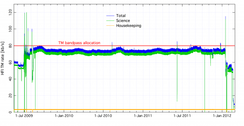
Optimal use of the bandpass available for the downlink was obtained initially by using a value of Q = σ/2.5 for all bolometer signals. After the 12th of December 2009, and only for the 857 GHz detectors, the value was reset to Q = σ/2.0 to avoid data loss due to exceeding the limit of the downlink rate. With these settings the load during the mission never exceeded the allowed bandpass width, as is seen on the next figure.

Setting the quantization step in flight[edit]
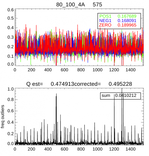
The only parameter that enters the Planck-HFI compression algorithm is the size of the quantization step, in units of , the white noise standard deviation for each channel. This quantity was adjusted during the mission by studying the mean frequency of the central quantization bin [-Q/2,Q/2], p0, within each compression slice (254 samples). For pure Gaussian noise, this frequency is related to the step size (in units of σ) by where the approximation is valid for p0<0.4. In Planck, however, the channel signal is not a pure Gaussian, since glitches and the periodic crossing of the Galactic plane add some strong outliers to the distribution. By using the frequency of these outliers above 5σ, pout}, simulations show that the following formula gives a valid estimate:
The following figure shows an example of the and timelines that were used to monitor and adjust the quantization setting.

Impact of the data compression on science[edit]
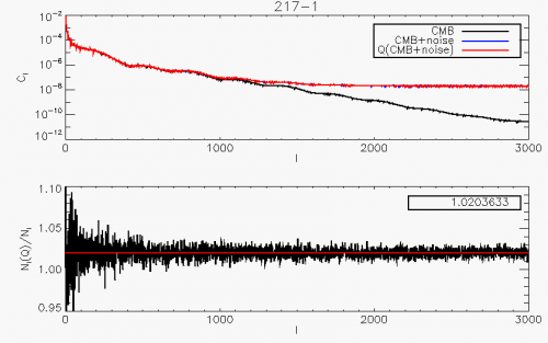
The effect of a pure quantization process of step Q (in units of σ) on the statistical moments of a signal is well known ([1]) When the step is typically below the noise level (which is largely the case for Planck) one can apply the Quantization Theorem which states that the process is equivalent to the addition of uniform random noise in the [-Q/2,Q/2] range. The net effect of quantization is therefore to add quadratically to the signal a Q2/12 variance. For Q≈0.5 this corresponds to a 2% noise level increase. The spectral effect of the non-linear quantization process is theoretically much more complicated and depends on the signal and noise details. As a rule of thumb, a pure quantization adds some auto-correlation function that is suppressed by a factor exp[-4π2(σ/Q)2] [2]. Note however that Planck does not perform a pure quantization process. A baseline is subtracted that depends on the data (specifically the mean of each compression slice value), is subtracted. Furthermore, for the science data, circles on the sky are coadded. Coaddition is again performed when projecting the rings onto the sky (map-making). To study the full effect of the Planck-HFI data compression algorithm on our main science products, we simulated a realistic data timeline, corresponding to the observation of a pure CMB sky. The compressed/decompressed signal was then back-projected onto the sky using the Planck scanning strategy. The two maps were analysed using the \texttt{anafast} HEALPix procedure and both reconstructed Cl were compared. The result is shown for a quantization step Q=0.5.

It is remarkable that the full procedure of
baseline-subtraction + quantization+ring-making + mapmaking still leads to the 2% increase of the
variance that is predicted by the simple timeline quantization (for Q/σ=2).
Furthermore we checked that the noise added by the compression algorithm is white.
It is not expected that the compression brings any non-Gaussianity, since the pure quantization process does not add any skewness and less than 0.001 kurtosis, and coaddition of circles and then rings erases any non-Gaussian contribution according to the central limit theorem.
References[edit]
- Jump up ↑ A Study of Rough Amplitude Quantization by Means of Nyquist Sampling Theory, B Widrow, IRE Transactions on Circuit Theory, CT-3(4), 266-276, (1956).
- Jump up ↑ On the autocorrelation function of quantized signal plus noise, E. Banta, Information Theory, IEEE Transactions on, 11, 114 - 117, (1965).
Readout Electronic Unit
analog to digital converter
Data Processing Unit
(Planck) High Frequency Instrument
Cosmic Microwave background
(Hierarchical Equal Area isoLatitude Pixelation of a sphere, <ref name="Template:Gorski2005">HEALPix: A Framework for High-Resolution Discretization and Fast Analysis of Data Distributed on the Sphere, K. M. Górski, E. Hivon, A. J. Banday, B. D. Wandelt, F. K. Hansen, M. Reinecke, M. Bartelmann, ApJ, 622, 759-771, (2005).