|
|
| (186 intermediate revisions by 13 users not shown) |
| Line 1: |
Line 1: |
| − | The inversion of HFI data requires that one knows how the instrument selects photons, how these photons are transformed in data transmitted by telemetry and what spurious signals are added in this process.
| + | This section provides an overview of the High-Frequency Instrument and of its different sub-systems. |
| − | [[Category:Instruments]]
| |
| | | | |
| − | ==HFI high level description and Architecture==
| + | * [[HFI_cryogenics | Cryogenics]] |
| | + | * [[HFI_cold_optics_%26_spectral_response | HFI cold optics and spectral response]] |
| | + | * [[HFI_detection_chain | Detection chain]] |
| | + | * [[HFI_operations | Operations]] |
| | + | * [[HFI_performance_summary | Performance summary]] |
| | + | * [[HFI_instrument_annexes | Annexes]] |
| | | | |
| − | <span style="color:red">(Lamarre/Pajot)</span>
| + | Two papers that include and detail this information are available: {{PlanckPapers|lamarre2010}} and {{PlanckPapers|planck2011-1-5}}. Additional detailed information potentially useful for users of HFI data is included in this section or annexed to it. |
| − | Should be short, understandable and point through links to the relevant sections and papers.
| |
| | | | |
| − | ==Cryogenics==
| + | [[Image:HFI_2_4_1_JML_TheElectronicsAndServiceModule.png|thumb|500px|center|HFI electronics in the satellite]] |
| − | <span style="color:red">(F .Pajot)</span>
| |
| − | ===Dilution===
| |
| | | | |
| − | (including PIDs) | + | The HFI instrument is designed around 52 bolometers. Twenty of the bolometers (spider-web bolometers or SWBs) are sensitive to total power, and the remaining 32 units are arranged in pairs of orthogonally-oriented polarisation-sensitive bolometers (PSBs). All bolometers are operated at a temperature of ~0.1 K by means of a space qualified dilution cooler coupled to a high precision temperature control system. A 4He-JT system provides active cooling for 4 K stages using vibration controlled mechanical compressors to prevent excessive warming of the 100 mK stage and minimize microphonic effects in the bolometers. Bolometers and sensitive thermometers are read using an AC-bias scheme through JFET amplifiers operated at ~130 K that provide high sensitivity and low frequency stability. The HFI covers six bands centred at 100, 143, 217, 353, 545, and 857 GHz, thanks to a thermo-optical design consisting of three corrugated horns and a set of compact reflective filters and lenses at cryogenic temperatures. |
| | | | |
| − | The HFI 3He-4He dilution cooler produces
| + | [[Image:HFI_horns.jpg|thumb|500px|center|HFI focal plane optics and 4K thermo-mechanical stage.]] |
| − | temperatures of 0.1 K for the bolometers through
| |
| − | the dilution of 3He into 4He and 1.4 K through JT
| |
| − | expansion of the 3He and 4He mixture. The
| |
| − | dilution cooler is described in detail in [Planck
| |
| − | early results. II. The thermal performance of
| |
| − | Planck, 2.3.3. Dilution cooler].
| |
| | | | |
| − | The dilution was operated with flows set to the | + | The whole satellite is organized to provide thermal transitions between its warm part exposed to radiation from the Sun and Earth, and the focal plane instruments that include the cold receivers (Sections [[HFI_cold_optics]] and [[HFI_detection_chain]]). The various parts of the HFI are distributed among three different stages of the satellite in order to provide each sub-system with an optimal operating temperature. The "warm" parts, including nearly all the electronics and the sources of fluids of the 4K and 0.1K coolers, are attached and thermally linked to the service module of the satellite. The first stage of the preamplifiers is attached to the back of the passively cooled telescope structure. The focal plane unit is attached to the 20K stage cooled by the sorption cooler. This is detailed in Section [[HFI_detection_chain]]. |
| − | minimum available value, and provided a total
| |
| − | lifetime of 30.5 months, exceeding the nominal
| |
| − | lifetime of 16 months by 14.5 months. The
| |
| − | dilution stage was stabilized by a PID control
| |
| − | with a power comprised between 20 and 30 nW
| |
| − | providing a temperature near 101 mK. The
| |
| − | bolometer plate was stabilized at 102.8 mK with a
| |
| − | PID power around 5 nW [fig. 100mK_stability.png].
| |
| | | | |
| − | (here a few lines of 100 mK boloplate stability)
| + | The telescope and horns select the geometrical origin of photons. They provide a high transmission efficiency to photons inside the main beam, while photons coming from the intermediate and far-side lobes have very low probability of being detected. The essential characteristics are determined by a complex process mixing ground measurements of components (horns, reflectors), modelling the shape of the far sidelobes, and measuring bright sources in-flight, especially planets. |
| | | | |
| − | Detailed of the in-flight performance of the
| + | The filters and bolometers define the spectral response and absolute optical efficiency, which are known mostly from ground-based measurements performed at component, sub-system, and system levels, reported in this document. The relationships between spectral response and geometrical response are also addressed. |
| − | dilution cooler can be found in [Planck early
| |
| − | results. II. The thermal performance of Planck,
| |
| − | 4.4. Dilution cooler]
| |
| | | | |
| − | === 4K J-T cooler ===
| + | Photons absorbed by a bolometer include the thermal radiation emitted by the various optical devices: telescope, horns, and filters. They are transformed into heat that propagates to the bolometer thermometer to influence its temperature, which is itself measured by the readout electronics. Temperatures of all these items must be stable enough not to contaminate the scientific signal delivered by the bolometers. How this stability is reached is described in Section [[HFI_cryogenics]]. |
| | | | |
| − | (including PIDs for details links to the early cryogenic paper (need to add data ?))
| + | The bolometer temperature depends also on the temperature of the bolometer plate, on the intensity of the biasing current, and on any spurious inputs, such as cosmic rays and mechanical vibrations. Such systematics are included in a list discussed in Section [[HFI-Validation]]. |
| | | | |
| − | The HFI 4K J-T cooler produces a temperature of
| + | Since the bolometer thermometer is part of an active circuit that also heats it, the response of this system is complex and has to be considered as a whole. In addition, due to the modulation of the bias current and to the sampling of the data, the response signal of the instrument when scanning a point source is more complex still. Item in Sub-Section [[HFI_detection_chain#Time_response|Time_response]] and Annex [[HFI_time_response_model]] are dedicated to the description of this time response. |
| − | 4K for the HFI 4K stage and optics and the
| |
| − | precooling of the dilution gases. Full
| |
| − | description of the 4K cooler can be found in
| |
| − | [Planck early results. II. The thermal | |
| − | performance of Planck, 2.3.2. 4He-JT cooler].
| |
| | | | |
| − | The 4K cooler was operated without interruption
| + | [[Image:HFI_2_4_1_JML_SignalFormation.png|thumb|500px|center|HFI signal formation.]] |
| − | during all the survey phase of the mission. It is
| |
| − | still in operation as it also provides the
| |
| − | cooling of the optical reference loads of the
| |
| − | LFI. The 4K PID stabilizing the temperature of
| |
| − | the HFI optics is regulated at 4.81 K using a
| |
| − | power around 1.8 mW [fig. 4K -A VENIR-].
| |
| | | | |
| − | (here a few lines of 4K stability, including compressors operation)
| + | Logic of the formation of the signal in HFI. This is an idealized description of the physics that takes place in the instrument. The optical power that is absorbed by the bolometers comes from the observed sky and from the instrument itself. The bolometers and readout electronics, acting as a single and complex chain, transform this optical power into data that are compressed and transmitted for science data reduction. |
| | | | |
| − | Details on the in-flight performance of the
| + | <div style="clear: both"></div> |
| − | dilution cooler can be found in [Planck early
| + | == References == |
| − | results. II. The thermal performance of Planck,
| + | <References /> |
| − | 4.3. 4He-JT cooler]
| + | |
| | + | |
| | | | |
| − | [[File:100mK_stability.png|500px|je ne sais pas quelle est la légende !]]
| |
| | | | |
| − | | + | [[Category:HFI design, qualification and performance|000]] |
| − | == Cold optics ==
| |
| − | <span style="color:red">(Lamarre)</span>
| |
| − | === Horns,lenses===
| |
| − | links to Peter's paper
| |
| − | === filters, band===
| |
| − | Includes Locke's very detailed document.
| |
| − | | |
| − | == Detection chain ==
| |
| − | <span style="color:red">(Francesco Piacentini)</span>
| |
| − | === Bolometers===
| |
| − | === JFETs===
| |
| − | === Readout===
| |
| − | === Data compression===
| |
| − | === Time response.===
| |
| − | Links to Brendan's paper. Additional data if needed. Written by Brendan.
| |
| − | | |
| − | The time response of the HFI bolometers and readout electronics is modelled as a Fourier domain transfer function (called the LFER4 model) consisting of the product of an bolometer thermal response <math>F(\omega)</math> and an electronics response <math>H'(\omega)</math>. <math>TF^{LFER4}(\omega) = F(\omega) H'(\omega)
| |
| − | </math>
| |
| − | | |
| − | In the processing of the HFI data, the time response is deconvolved (see TOI processing section).
| |
| − | | |
| − | === LFER4 model ===
| |
| − | | |
| − | If we write the input signal (power) on a bolometer as <math>\label{bol_in}
| |
| − | s_0(t)=e^{i\omega t}
| |
| − | </math> the bolometer physical impedance can be written as: <math>\label{bol_out}
| |
| − | s(t)=e^{i\omega t}F(\omega)
| |
| − | </math> where <math>\omega</math> is the angular frequency of the signal and <math>F(\omega)</math> is the complex intrinsic bolometer transfer function. For HFI the bolometer transfer function is modelled as the sum of 4 single pole low pass filters: <math>\label{bol_tf}
| |
| − | F(\omega) = \sum_{i=0,4} \frac{a_i}{1 + i\omega\tau_i}
| |
| − | </math> The modulation of the signal is done with a square wave, written here as a composition of sine waves of decreasing amplitude: <math>\label{sigmod}
| |
| − | s'(t)=e^{i\omega t}F(\omega)\sum_{k=0}^{\infty} \frac{e^{i\omega_r(2k+1)t}-e^{-i\omega_r(2k+1)t}}{2i(2k+1)}
| |
| − | </math> where we have used the Euler relation <math>\sin x=(e^{ix}-e^{-ix})/2i</math> and <math>\omega_r</math> is the angular frequency of the square wave. The modulation frequency is <math>f_{mod} = \omega_r/2\pi</math> and was set to <math>f_{mod} = 90.18759 </math>Hz in flight. This signal is then filtered by the complex electronic transfer function <math>H(\omega)</math>. Setting: <math>\omega_k^+=\omega+(2k+1)\omega_r</math> <math>\omega_k^-=\omega-(2k+1)\omega_r</math> we have: <math>\label{sigele}
| |
| − | \Sigma(t)=\sum_{k=0}^\infty\frac{F(\omega)}{2i(2k+1)}\left[H(\omega_k^+)e^{i\omega_k^+t}-H(\omega_k^-)e^{i\omega_k^-t}\right]
| |
| − | </math> This signal is then sampled at high frequency (<math>2 f_{mod} NS</math>). <math>NS</math> is one of the parameters of the HFI electronics and corresponds to the number of high frequency samples in each modulation semi-period. In order to obtain an output signal sampled every <math>\pi/\omega_r</math> seconds, we must integrate on a semiperiod, as done in the HFI readout. To also include a time shift <math>\Delta t</math>, the integral is calculated between <math>n\pi/\omega_r+\Delta t</math> and <math>(n+1)\pi/\omega_r+\Delta t</math> (with <math>T=2 \pi/\omega_r</math> period of the modulation). The time shift <math>\Delta t</math> is encoded in the HFI electronics by the parameter <math>S_{phase}</math>, with the relation <math>\Delta t = S_{phase}/NS/f_{mod} </math>.
| |
| − | | |
| − | After integration, the <math>n</math>-sample of a bolometer can be written as <math>\label{eqn:output}
| |
| − | Y(t_n) = (-1)^n F(\omega) H'(\omega) e^{i t_n \omega}
| |
| − | </math> where <math>\label{tfele}
| |
| − | H'(\omega) = \frac 12 \sum_{k=0}^\infty
| |
| − | e^{-i(\frac{\pi\omega}{2\omega_r}+\omega\Delta t)} \Bigg[
| |
| − | \frac{H(\omega_k^+)e^{i\omega_k^+ \Delta t}}{(2k+1)\omega_k^+}
| |
| − | \left(1-e^{\frac{i\omega_k^+\pi}{\omega_r}}\right)
| |
| − | \\ - \frac{H(\omega_k^-)e^{i\omega_k^- \Delta t}}{(2k+1)\omega_k^-} \left(1-e^{\frac{i\omega_k^-\pi}{\omega_r}}\right)
| |
| − | \Bigg]
| |
| − | </math>
| |
| − | | |
| − | The output signal in equation eqn:output can be demodulated (thus removing the <math>(-1)^n</math>) and compared to the input signal in equation bol_in. The overall transfer function is composed of the bolometer transfer function and the effective electronics transfer function, <math>H'(\omega)</math>: <math>TF(\omega) = F(\omega) H'(\omega)
| |
| − | </math>
| |
| − | | |
| − | The shape of <math>H(\omega)</math> is obtained combining low and high-pass filters with Sallen Key topologies (with their respective time constants) and accounting also for the stray capacitance low pass filter given by the bolometer impedance combined with the stray capacitance of the cables. The sequence of filters that define the electronic band-pass function <math>H(\omega) = h_0*h_1*h_2*h_3*h_4*h_{5}</math> are listed in table table:readout_electronics_filters.
| |
| − | | |
| − | === Parameters of LFER4 model ===
| |
| − | | |
| − | The LFER4 model has are a total of 10 parameters, 9 of which are independent, for each bolometer. The free parameters of the LFER4 model are determined using in-flight data in the following ways:
| |
| − | | |
| − | {itemize}
| |
| − | <math>S_{phase}</math> is fixed at the value of the REU setting.
| |
| − | | |
| − | <math>\tau_{stray}</math> is measured during the QEC test during CPV.
| |
| − | | |
| − | <math>A_1</math>, <math>\tau_1</math>, <math>A_2</math>, <math>\tau_2</math> are fit forcing the compactness of the scanning beam.
| |
| − | | |
| − | <math>A_3</math>, <math>\tau_3</math>, <math>A_{4}</math> <math>\tau_4</math> are fit by forcing agreement of survey 2 and survey 1 maps.
| |
| − | | |
| − | the overall normalization of the LFER4 model is forced to be 1.0 at the signal frequency of the dipole.
| |
| − | | |
| − | {\itemize}
| |
| − | The details of determining the model parameters are given in (reference P03c paper) and the best-fit parameters listed here in table table:LFER4pars.
| |
| − | | |
| − | <blockquote>
| |
| − | | |
| − | =5pt {HFI electronics filter sequence. We define $s = i \omega$.}
| |
| − | | |
| − | | |
| − | (table:readout_electronics_filters)
| |
| − | | |
| − | | |
| − | -3mm ={
| |
| − | \newdimen\digitwidth
| |
| − | \setbox0=\hbox{\rm 0}
| |
| − | \digitwidth=\wd0
| |
| − | \catcode`*=\active
| |
| − | \def*{\kern\digitwidth}
| |
| − | %
| |
| − | \newdimen\signwidth
| |
| − | \setbox0=\hbox{+}
| |
| − | \signwidth=\wd0
| |
| − | \catcode`!=\active
| |
| − | \def!{\kern\signwidth}
| |
| − | %
| |
| − | \halign{#\tabskip 2em&
| |
| − | \vtop{\hsize 1.5in\noindent\strut#\strut\par}\tabskip 2em &
| |
| − | \vtop{\hsize 2.0in\noindent\strut#\strut\par}\tabskip 2em&
| |
| − | \vtop{\hsize 1.5in\noindent\strut#\strut\par}\cr % Template goes here.
| |
| − | \noalign{\doubleline}
| |
| − | % Table headings go here.
| |
| − | &Filter& Parameters&Function\cr
| |
| − | \noalign{\vskip 3pt\hrule\vskip 5pt}
| |
| − | % Body of table goes here
| |
| − | 0&Stray capacitance low pass filter& $\tau_{stray}= R_{bolo}
| |
| − | C_{stray}$ & $h_0 = \frac{1}{1.0+\tau_{stray}*s}$\cr
| |
| − | 1&Low pass filter& $R_1=1$k$\Omega$ \\
| |
| − | $C_1=100$nF & $h_1 = \frac{2.0+R_1*C_1*s}{2.0*(1.0+R_1*C_1*s)}$\cr
| |
| − | 2&Sallen Key high pass filter &$R_2=51$k$\Omega$\\
| |
| − | $C_2=1\mu$F&$h_2= \frac{(R_2*C_2*s)^2}{(1.0+R_2*C_2*s)^2}$\cr
| |
| − | 3&Sign reverse with gain &&$h_3=-5.1$\cr
| |
| − | 4&Single pole low pass filter with gain &$R_4=10$k$\Omega$\\
| |
| − | $C_4=10$nF&$h_4= \frac{1.5}{1.0+R_4*C_4*s}$\cr
| |
| − | 5&Single pole high pass filter coupled to a
| |
| − | Sallen Key low pass filter&$R_9=18.7$k$\Omega$\\
| |
| − | $R_{12}=37.4$k$\Omega$\\
| |
| − | $C=10.0$nF\\
| |
| − | $R_{78}=510$k$\Omega$\\
| |
| − | $C_{18}=1.0\mu$F\\
| |
| − | $K_3 = R_9^2*R_{78}*R_{12}^2*C^2*C_{18}$\\
| |
| − | $K_2 = R_9*R_{12}^2*R_{78}*C^2+R_{9}^2*R_{12}^2*C^2+R_9*R_{12}^2*R_{78}*C_{18}*C$\\
| |
| − | $K_1 =R_9*R_{12}^2*C+R_{12}*R_{78}*R_9*C_{18}$&$h_{5} = \frac{2.0*R_{12}*R_9*R_{78}*C_{18}*s}{s^3*K_3 +
| |
| − | s^2*K_2+
| |
| − | s*K_1 + R_{12}*R_9 } $\cr
| |
| − | \noalign{\vskip 5pt\hrule\vskip 3pt}}}
| |
| − | | |
| − | | |
| − | | |
| − | | |
| − | </blockquote>
| |
| − | <blockquote>
| |
| − | | |
| − | =5pt {Parameters for LFER4 model that are deconvolved from the data.}
| |
| − | | |
| − | | |
| − | (table:LFER4pars)
| |
| − | | |
| − | | |
| − | -3mm ={
| |
| − | \newdimen\digitwidth
| |
| − | \setbox0=\hbox{\rm 0}
| |
| − | \digitwidth=\wd0
| |
| − | \catcode`*=\active
| |
| − | \def*{\kern\digitwidth}
| |
| − | %
| |
| − | \newdimen\signwidth
| |
| − | \setbox0=\hbox{+}
| |
| − | \signwidth=\wd0
| |
| − | \catcode`!=\active
| |
| − | \def!{\kern\signwidth}
| |
| − | %
| |
| − | \halign{#\hfil \tabskip 2em&\hfil# \tabskip 1em&#\hfil \tabskip 1em &\hfil# \tabskip 1em&\hfil# \tabskip 1em&\hfil# \tabskip 1em&\hfil# \tabskip 1em&\hfil# \tabskip 1em&\hfil# \tabskip 1em&\hfil# \tabskip 1em&\hfil# \tabskip 1em\cr % Template goes here.
| |
| − | \noalign{\doubleline}
| |
| − | % Table headings go here.
| |
| − | Bolometer&$A_1$&$\tau_1$&$A_2$&$\tau_2$&$A_3$&$\tau_3$&$A_4$&$\tau_4$&$\tau_{stray}$&$S_{phase}$\cr
| |
| − | & & ms & & ms & & ms & &ms& ms &\cr
| |
| − | \noalign{\vskip 3pt\hrule\vskip 5pt}
| |
| − | % Body of table goes here.
| |
| − | 100-1a&0.392& 10&0.534&20.9&0.0656&51.3&0.00833& 572&1.59&0.00139\cr
| |
| − | 100-1b&0.484&10.3&0.463&19.2&0.0451&71.4&0.00808& 594&1.49&0.00139\cr
| |
| − | 100-2a&0.474&6.84&0.421&13.6&0.0942&37.6&0.0106& 346&1.32&0.00125\cr
| |
| − | 100-2b&0.126&5.84&0.717&15.1&0.142&35.1&0.0145& 293&1.38&0.00125\cr
| |
| − | 100-3a&0.744&5.39&0.223&14.7&0.0262&58.6&0.00636& 907&1.42&0.00125\cr
| |
| − | 100-3b&0.608&5.48&0.352&15.5&0.0321&63.6&0.00821& 504&1.66&0.00125\cr
| |
| − | 100-4a&0.411& 8.2&0.514&17.8&0.0581&57.9&0.0168& 370&1.25&0.00125\cr
| |
| − | 100-4b&0.687&11.3&0.282&24.3&0.0218& 62&0.00875& 431&1.38&0.00139\cr
| |
| − | 143-1a&0.817&4.47&0.144&12.1&0.0293&38.7&0.0101& 472&1.42&0.00125\cr
| |
| − | 143-1b&0.49&4.72&0.333&15.6&0.134&48.1&0.0435& 270&1.49&0.00125\cr
| |
| − | 143-2a&0.909& 4.7&0.0763& 17&0.00634& 100&0.00871& 363&1.48&0.00125\cr
| |
| − | 143-2b&0.912&5.24&0.0509&16.7&0.0244&26.5&0.0123& 295&1.46&0.00125\cr
| |
| − | 143-3a&0.681&4.19&0.273&9.56&0.0345&34.8&0.0115& 317&1.45&0.00125\cr
| |
| − | 143-3b&0.82&4.48&0.131&13.2&0.0354&35.1&0.0133& 283&1.61&0.000832\cr
| |
| − | 143-4a&0.914&5.69&0.072&18.9&0.00602&48.2&0.00756& 225&1.59&0.00125\cr
| |
| − | 143-4b&0.428&6.06&0.508&6.06&0.0554&22.7&0.00882& 84&1.82&0.00125\cr
| |
| − | 143-5&0.491&6.64&0.397&6.64&0.0962&26.4&0.0156& 336&2.02&0.00139\cr
| |
| − | 143-6&0.518&5.51&0.409&5.51&0.0614&26.6&0.0116& 314&1.53&0.00111\cr
| |
| − | 143-7&0.414&5.43&0.562&5.43&0.0185&44.9&0.00545& 314&1.86&0.00139\cr
| |
| − | 217-5a&0.905&6.69&0.0797&21.6&0.00585&65.8&0.00986& 342&1.57&0.00111\cr
| |
| − | 217-5b&0.925&5.76&0.061& 18&0.00513&65.6&0.0094& 287&1.87&0.00125\cr
| |
| − | 217-6a&0.844&6.45&0.0675&19.7&0.0737&31.6&0.0147& 297&1.54&0.00125\cr
| |
| − | 217-6b&0.284&6.23&0.666&6.23&0.0384& 24&0.0117& 150&1.46&0.00111\cr
| |
| − | 217-7a&0.343&5.48&0.574&5.48&0.0717& 23&0.0107& 320&1.52&0.00139\cr
| |
| − | 217-7b&0.846&5.07&0.127&14.4&0.0131&47.9&0.0133& 311&1.51&0.00139\cr
| |
| − | 217-8a&0.496&7.22&0.439&7.22&0.0521&32.5&0.0128& 382&1.79&0.00111\cr
| |
| − | 217-8b&0.512&7.03&0.41&7.03&0.0639&27.2&0.0139& 232&1.73&0.00125\cr
| |
| − | 217-1&0.0136&3.46&0.956&3.46&0.0271&23.3&0.00359&1.98e+03&1.59&0.00111\cr
| |
| − | 217-2&0.978&3.52&0.014&26.1&0.00614& 42&0.00194& 686& 1.6&0.00125\cr
| |
| − | 217-3&0.932&3.55&0.0336&3.55&0.0292&32.4&0.00491& 279&1.74&0.00125\cr
| |
| − | 217-4&0.658&1.35&0.32&5.55&0.0174&26.8&0.00424& 473&1.71&0.00111\cr
| |
| − | 353-3a&0.554&7.04&0.36&7.04&0.0699&30.5&0.0163& 344& 1.7&0.00125\cr
| |
| − | 353-3b&0.219&2.68&0.671&6.95&0.0977&23.8&0.0119& 289&1.57&0.00111\cr
| |
| − | 353-4a&0.768&4.73&0.198&9.93&0.0283&50.5&0.00628& 536&1.81&0.00125\cr
| |
| − | 353-4b&0.684&4.54&0.224&10.8&0.0774& 80&0.0149& 267&1.66&0.00111\cr
| |
| − | 353-5a&0.767&5.96&0.159&12.4&0.0628&30.3&0.0109& 357&1.56&0.00111\cr
| |
| − | 353-5b&0.832&6.19&0.126&11.1&0.0324& 35&0.0096& 397&1.66&0.00111\cr
| |
| − | 353-6a&0.0487&1.76&0.855& 6&0.0856&21.6&0.0105& 222&1.99&0.00125\cr
| |
| − | 353-6b&0.829&5.61&0.127&5.61&0.0373&25.2&0.00696& 360&2.28&0.00111\cr
| |
| − | 353-1&0.41&0.743&0.502&4.22&0.0811&17.7&0.0063& 329&1.32&0.00097\cr
| |
| − | 353-2&0.747&3.09&0.225&7.26&0.0252&44.7&0.00267& 513&1.54&0.00097\cr
| |
| − | 353-7&0.448& 0.9&0.537& 4.1&0.0122&27.3&0.00346& 433&1.78&0.00125\cr
| |
| − | 353-8&0.718&2.23&0.261&6.08&0.0165& 38&0.00408& 268&1.77&0.00111\cr
| |
| − | 545-1&0.991&2.93&0.00743& 26&0.00139&2.6e+03& & &2.16&0.00111\cr
| |
| − | 545-2&0.985&2.77&0.0128& 24&0.00246&2.8e+03& & &1.87&0.00097\cr
| |
| − | 545-4&0.972& 3&0.0277& 25&0.000777&2.5e+03& & &2.22&0.00111\cr
| |
| − | 857-1&0.974&3.38&0.0229& 25&0.00349&2.2e+03& & &1.76&0.00111\cr
| |
| − | 857-2&0.84&1.48&0.158&6.56&0.00249&3.2e+03& & & 2.2&0.00125\cr
| |
| − | 857-3&0.36&0.0422&0.627& 2.4&0.0111& 17&0.002&1.9e+03&1.52&0.00126\cr
| |
| − | 857-4&0.278& 0.4&0.719&3.92&0.00162& 90&0.00152& 800&1.49&0.000558\\\cr
| |
| − | \cr
| |
| − | \noalign{\vskip 3pt\hrule\vskip 5pt}
| |
| − | }
| |
| − | }
| |
| − | | |
| − | </blockquote>
| |
| − | | |
| − | | |
| − | == System (Ken) ==
| |
| − | ===List of systematics===
| |
| − | | |
| − | ==Summary==
| |
| − | <span style="color:red">(Lamarre)</span>
| |
| − | here remind worse sytematics and point to DPC
| |
| − | Summary of sucess and limitations. JML. Link to early HFI in flight perf.
| |
This section provides an overview of the High-Frequency Instrument and of its different sub-systems.
Two papers that include and detail this information are available: Planck-PreLaunch-IX[1] and Planck-Early-IV[2]. Additional detailed information potentially useful for users of HFI data is included in this section or annexed to it.
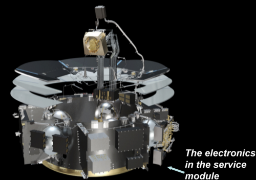
HFI electronics in the satellite
The HFI instrument is designed around 52 bolometers. Twenty of the bolometers (spider-web bolometers or SWBs) are sensitive to total power, and the remaining 32 units are arranged in pairs of orthogonally-oriented polarisation-sensitive bolometers (PSBs). All bolometers are operated at a temperature of ~0.1 K by means of a space qualified dilution cooler coupled to a high precision temperature control system. A 4He-JT system provides active cooling for 4 K stages using vibration controlled mechanical compressors to prevent excessive warming of the 100 mK stage and minimize microphonic effects in the bolometers. Bolometers and sensitive thermometers are read using an AC-bias scheme through JFET amplifiers operated at ~130 K that provide high sensitivity and low frequency stability. The HFI covers six bands centred at 100, 143, 217, 353, 545, and 857 GHz, thanks to a thermo-optical design consisting of three corrugated horns and a set of compact reflective filters and lenses at cryogenic temperatures.
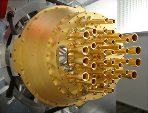
HFI focal plane optics and 4K thermo-mechanical stage.
The whole satellite is organized to provide thermal transitions between its warm part exposed to radiation from the Sun and Earth, and the focal plane instruments that include the cold receivers (Sections HFI_cold_optics and HFI_detection_chain). The various parts of the HFI are distributed among three different stages of the satellite in order to provide each sub-system with an optimal operating temperature. The "warm" parts, including nearly all the electronics and the sources of fluids of the 4K and 0.1K coolers, are attached and thermally linked to the service module of the satellite. The first stage of the preamplifiers is attached to the back of the passively cooled telescope structure. The focal plane unit is attached to the 20K stage cooled by the sorption cooler. This is detailed in Section HFI_detection_chain.
The telescope and horns select the geometrical origin of photons. They provide a high transmission efficiency to photons inside the main beam, while photons coming from the intermediate and far-side lobes have very low probability of being detected. The essential characteristics are determined by a complex process mixing ground measurements of components (horns, reflectors), modelling the shape of the far sidelobes, and measuring bright sources in-flight, especially planets.
The filters and bolometers define the spectral response and absolute optical efficiency, which are known mostly from ground-based measurements performed at component, sub-system, and system levels, reported in this document. The relationships between spectral response and geometrical response are also addressed.
Photons absorbed by a bolometer include the thermal radiation emitted by the various optical devices: telescope, horns, and filters. They are transformed into heat that propagates to the bolometer thermometer to influence its temperature, which is itself measured by the readout electronics. Temperatures of all these items must be stable enough not to contaminate the scientific signal delivered by the bolometers. How this stability is reached is described in Section HFI_cryogenics.
The bolometer temperature depends also on the temperature of the bolometer plate, on the intensity of the biasing current, and on any spurious inputs, such as cosmic rays and mechanical vibrations. Such systematics are included in a list discussed in Section HFI-Validation.
Since the bolometer thermometer is part of an active circuit that also heats it, the response of this system is complex and has to be considered as a whole. In addition, due to the modulation of the bias current and to the sampling of the data, the response signal of the instrument when scanning a point source is more complex still. Item in Sub-Section Time_response and Annex HFI_time_response_model are dedicated to the description of this time response.
Logic of the formation of the signal in HFI. This is an idealized description of the physics that takes place in the instrument. The optical power that is absorbed by the bolometers comes from the observed sky and from the instrument itself. The bolometers and readout electronics, acting as a single and complex chain, transform this optical power into data that are compressed and transmitted for science data reduction.
References[edit]
- ↑ Planck pre-launch status: The HFI instrument, from specification to actual performance, J.-M. Lamarre, J.-L. Puget, P. A. R. Ade, et al. , A&A, 520, A9+, (2010).
- ↑ Planck early results, IV. First assessment of the High Frequency Instrument in-flight performance, Planck HFI Core Team, A&A, 536, A4, (2011).


