Difference between revisions of "HFI-Validation"
m |
|||
| (163 intermediate revisions by 9 users not shown) | |||
| Line 1: | Line 1: | ||
| − | + | {{DISPLAYTITLE:Overall internal validation}} | |
| − | + | The overall internal validation of the frequency maps is performed thanks to several tests: | |
| + | * difference between the PR2 (2015) and PR3 (2018) frequency maps, | ||
| + | * survey difference maps for the PR2 and the PR3 frequency maps, | ||
| + | * spectra of the PR2 and the PR3 data splits, | ||
| + | * comparison of the FFP10 simulations and the PR3 data. | ||
| − | + | <br> | |
| + | <span style="font-size:150%">'''Frequency maps for the PR2 and the PR3 and their difference''' </span> | ||
| − | + | This table shows the PR2 and PR3 maps and their differences in I, Q, and U. This table is complementary of the figure in {{PlanckPapers|planck2016-l03}} (see detailled explanations there). | |
| − | + | {| border="1" cellpadding="3" cellspacing="0" align="center" style="text-align:centert" width=800px | |
| + | |+ '''Comparaison of PR2 and PR3 I, Q and U maps and their difference. ''' | ||
| + | |- bgcolor="ffdead" | ||
| + | ! | ||
| + | !colspan="3"| PR2 frequency maps | ||
| + | !colspan="3"| PR3 frequency maps | ||
| + | !colspan="3"| difference | ||
| + | |- | ||
| + | ! | ||
| + | !I | ||
| + | !Q | ||
| + | !U | ||
| + | !I | ||
| + | !Q | ||
| + | !U | ||
| + | !I | ||
| + | !Q | ||
| + | !U | ||
| + | |- | ||
| + | | 100 GHz | ||
| + | |[[File:100GHz_DX11_I.pdf.pdf|100px]] | ||
| + | |[[File:100GHz_DX11_Q.pdf.pdf|100px]] | ||
| + | |[[File:100GHz_DX11_U.pdf.pdf|100px]] | ||
| + | |[[File:100GHz_I.pdf|100px]] | ||
| + | |[[File:100GHz_Q.pdf|100px]] | ||
| + | |[[File:100GHz_U.pdf|100px]] | ||
| + | |[[File:100GHz_diff_I.pdf.pdf|100px]] | ||
| + | |[[File:100GHz_diff_Q.pdf.pdf|100px]] | ||
| + | |[[File:100GHz_diff_U.pdf.pdf|100px]] | ||
| + | |- | ||
| + | | 143 GHz | ||
| + | |[[File:143GHz_DX11_I.pdf.pdf|100px]] | ||
| + | |[[File:143GHz_DX11_Q.pdf.pdf|100px]] | ||
| + | |[[File:143GHz_DX11_U.pdf.pdf|100px]] | ||
| + | |[[File:143GHz_I.pdf|100px]] | ||
| + | |[[File:143GHz_Q.pdf|100px]] | ||
| + | |[[File:143GHz_U.pdf|100px]] | ||
| + | |[[File:143GHz_diff_I.pdf.pdf|100px]] | ||
| + | |[[File:143GHz_diff_Q.pdf.pdf|100px]] | ||
| + | |[[File:143GHz_diff_U.pdf.pdf|100px]] | ||
| + | |- | ||
| + | | 217 GHz | ||
| + | |[[File:217GHz_DX11_I.pdf.pdf|100px]] | ||
| + | |[[File:217GHz_DX11_Q.pdf.pdf|100px]] | ||
| + | |[[File:217GHz_DX11_U.pdf.pdf|100px]] | ||
| + | |[[File:217GHz_I.pdf|100px]] | ||
| + | |[[File:217GHz_Q.pdf|100px]] | ||
| + | |[[File:217GHz_U.pdf|100px]] | ||
| + | |[[File:217GHz_diff_I.pdf.pdf|100px]] | ||
| + | |[[File:217GHz_diff_Q.pdf.pdf|100px]] | ||
| + | |[[File:217GHz_diff_U.pdf.pdf|100px]] | ||
| + | |- | ||
| + | | 353 GHz | ||
| + | |[[File:353GHz_DX11_I.pdf.pdf|100px]] | ||
| + | |[[File:353GHz_DX11_Q.pdf.pdf|100px]] | ||
| + | |[[File:353GHz_DX11_U.pdf.pdf|100px]] | ||
| + | |[[File:353GHz_I.pdf|100px]] | ||
| + | |[[File:353GHz_Q.pdf|100px]] | ||
| + | |[[File:353GHz_U.pdf|100px]] | ||
| + | |[[File:353GHz_diff_I.pdf.pdf|100px]] | ||
| + | |[[File:353GHz_diff_Q.pdf.pdf|100px]] | ||
| + | |[[File:353GHz_diff_U.pdf.pdf|100px]] | ||
| + | |- | ||
| + | | 545 GHz | ||
| + | |[[File:545GHz_DX11_I.pdf.pdf|100px]] | ||
| + | | . | ||
| + | | . | ||
| + | |[[File:545GHz_I.pdf|100px]] | ||
| + | | . | ||
| + | | . | ||
| + | |[[File:545GHz_diff_I.pdf.pdf|100px]] | ||
| + | | . | ||
| + | | . | ||
| + | |- | ||
| + | | 857 GHz | ||
| + | |[[File:857GHz_DX11_I.pdf.pdf|100px]] | ||
| + | | . | ||
| + | | . | ||
| + | |[[File:857GHz_I.pdf|100px]] | ||
| + | | . | ||
| + | | . | ||
| + | |[[File:857GHz_diff_I.pdf.pdf|100px]] | ||
| + | | . | ||
| + | | . | ||
| + | |} | ||
| − | |||
| − | + | <br> | |
| + | <span style="font-size:150%">'''Survey difference maps for the PR2 and the PR3 data''' </span> | ||
| − | + | This table shows the PR2 and PR3 survey difference maps ((S1+S3)-(S2+S4))in I, Q, and U. This table is taken from {{PlanckPapers|planck2016-l03}} (see detailled explanations there). | |
| − | [[ | + | {| border="1" cellpadding="3" cellspacing="0" align="center" style="text-align:centert" width=800px |
| − | + | |+ '''Comparaison of PR2 and PR3 I, Q and U survey difference maps.''' | |
| + | |- bgcolor="ffdead" | ||
| + | ! | ||
| + | !colspan="3"| PR2 survey difference maps | ||
| + | !colspan="3"| PR3 survey difference maps | ||
| + | |- | ||
| + | ! | ||
| + | !I | ||
| + | !Q | ||
| + | !U | ||
| + | !I | ||
| + | !Q | ||
| + | !U | ||
| + | |- | ||
| + | | 100 GHz | ||
| + | |[[File:100GHz_DX11_surveyS1S3_S2S4_I.pdf|100px]] | ||
| + | |[[File:100GHz_DX11_surveyS1S3_S2S4_Q.pdf.pdf|100px]] | ||
| + | |[[File:100GHz_DX11_surveyS1S3_S2S4_U.pdf.pdf|100px]] | ||
| + | |[[File:100GHz_RD12RC4_surveyS1S3_S2S4_I.pdf|100px]] | ||
| + | |[[File:100GHz_RD12RC4_surveyS1S3_S2S4_Q.pdf|100px]] | ||
| + | |[[File:100GHz_RD12RC4_surveyS1S3_S2S4_U.pdf|100px]] | ||
| + | |- | ||
| + | | 143 GHz | ||
| + | |[[File:143GHz_DX11_surveyS1S3_S2S4_I.pdf|100px]] | ||
| + | |[[File:143GHz_DX11_surveyS1S3_S2S4_Q.pdf.pdf|100px]] | ||
| + | |[[File:143GHz_DX11_surveyS1S3_S2S4_U.pdf.pdf|100px]] | ||
| + | |[[File:143GHz_RD12RC4_surveyS1S3_S2S4_I.pdf|100px]] | ||
| + | |[[File:143GHz_RD12RC4_surveyS1S3_S2S4_Q.pdf|100px]] | ||
| + | |[[File:143GHz_RD12RC4_surveyS1S3_S2S4_U.pdf|100px]] | ||
| + | |- | ||
| + | | 217 GHz | ||
| + | |[[File:217GHz_DX11_surveyS1S3_S2S4_I.pdf|100px]] | ||
| + | |[[File:217GHz_DX11_surveyS1S3_S2S4_Q.pdf.pdf|100px]] | ||
| + | |[[File:217GHz_DX11_surveyS1S3_S2S4_U.pdf.pdf|100px]] | ||
| + | |[[File:217GHz_RD12RC4_surveyS1S3_S2S4_I.pdf|100px]] | ||
| + | |[[File:217GHz_RD12RC4_surveyS1S3_S2S4_Q.pdf|100px]] | ||
| + | |[[File:217GHz_RD12RC4_surveyS1S3_S2S4_U.pdf|100px]] | ||
| + | |- | ||
| + | | 353 GHz | ||
| + | |[[File:353GHz_DX11_surveyS1S3_S2S4_I.pdf|100px]] | ||
| + | |[[File:353GHz_DX11_surveyS1S3_S2S4_Q.pdf.pdf|100px]] | ||
| + | |[[File:353GHz_DX11_surveyS1S3_S2S4_U.pdf.pdf|100px]] | ||
| + | |[[File:353GHz_RD12RC4_surveyS1S3_S2S4_I.pdf|100px]] | ||
| + | |[[File:353GHz_RD12RC4_surveyS1S3_S2S4_Q.pdf|100px]] | ||
| + | |[[File:353GHz_RD12RC4_surveyS1S3_S2S4_U.pdf|100px]] | ||
| + | |- | ||
| + | | 545 GHz | ||
| + | |[[File:545GHz_DX11_surveyS1S3_S2S4_I.pdf|100px]] | ||
| + | | . | ||
| + | | . | ||
| + | |[[File:545GHz_RD12RC4_surveyS1S3_S2S4_I.pdf|100px]] | ||
| + | | . | ||
| + | | . | ||
| + | |- | ||
| + | | 857 GHz | ||
| + | |[[File:857GHz_DX11_surveyS1S3_S2S4_I.pdf|100px]] | ||
| + | | . | ||
| + | | . | ||
| + | |[[File:857GHz_RD12RC4_surveyS1S3_S2S4_I.pdf|100px]] | ||
| + | | . | ||
| + | | . | ||
| + | |} | ||
| − | + | <br> | |
| + | <span style="font-size:150%">'''Spectra of the PR2 and the PR3 data splits''' </span> | ||
| − | ===< | + | This figure shows the ''EE'' and ''BB'' spectra of the PR2 and PR3 detset, half-mission and rings (for PR3 only) maps at 100, 143, 217, and 353 GHz. The auto-spectra of the difference maps and the cross-spectra between the maps are shown. The sky fraction used here is 43 %. The bins are: bin=1 for <math>2\leq\ell<30</math>; bin=5 for <math>30\leq\ell<50</math>; bin=10 for <math>50\leq\ell<160</math>; bin=20 for <math>160\leq\ell<1000</math>; and bin=100 for <math>\ell>1000</math>. This figure is taken from {{PlanckPapers|planck2016-l03}} (see detailled explanations there). |
| − | + | <center> | |
| + | [[File:cl_fsky43_DX11_RD12RC4_3000_oddeven_multiplot.pdf|500px]] | ||
| + | </center> | ||
| − | |||
| − | |||
| − | |||
| − | |||
| − | |||
| − | |||
| − | |||
| − | |||
| − | |||
| − | |||
| − | + | <br> | |
| + | <span style="font-size:150%">'''Comparison of the FFP10 simulated noise and systematic residuals and the PR3 data''' </span> | ||
| − | + | This figure shows the noise and systematic residuals in ''TT'', ''EE'', ''BB'', and ''EB'' spectra, at the three CMB frequencies, for difference maps of the ring (red) and half-mission (blue) null tests binned by <math>\Delta \ell =10</math>. Data spectra are represented by thick lines, and the averages of simulations by thin black lines. For the simulations, we show the 16 % and 84 % quantiles of the distribution with the same colours. This figure is taken from {{PlanckPapers|planck2016-l03}} (see detailled explanations there). | |
| − | + | <center> | |
| + | [[File:newpte.pdf|500px]] | ||
| + | </center> | ||
| − | |||
| − | |||
| − | |||
| − | |||
| − | |||
| − | |||
| − | |||
| + | ==References== | ||
| − | + | <References /> | |
| − | + | ||
| − | |||
| − | |||
| − | |||
| − | |||
| − | |||
| − | |||
| − | |||
| − | |||
| − | |||
| − | |||
| − | |||
| − | |||
| − | |||
| − | |||
| − | |||
| − | |||
| − | |||
| − | |||
| − | |||
| − | |||
| − | |||
| − | |||
| − | |||
| − | |||
| − | |||
| − | |||
| − | |||
| − | |||
| − | |||
| − | |||
| − | |||
| − | |||
| − | |||
| − | |||
| − | |||
| − | |||
| − | |||
| − | |||
| − | |||
| − | |||
| − | |||
| − | |||
| − | + | [[Category:HFI data processing|006]] | |
Latest revision as of 08:40, 3 July 2018
The overall internal validation of the frequency maps is performed thanks to several tests:
- difference between the PR2 (2015) and PR3 (2018) frequency maps,
- survey difference maps for the PR2 and the PR3 frequency maps,
- spectra of the PR2 and the PR3 data splits,
- comparison of the FFP10 simulations and the PR3 data.
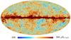
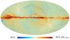
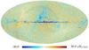
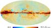
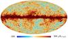
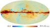
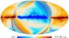
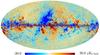
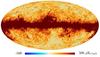
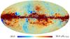
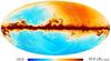
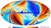
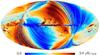
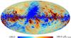
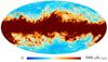
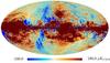
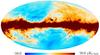
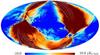
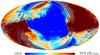
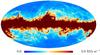
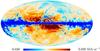
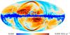
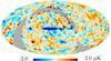
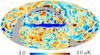
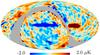
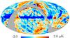
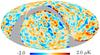
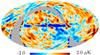
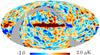
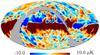
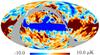
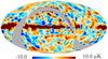
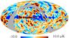
Frequency maps for the PR2 and the PR3 and their difference
This table shows the PR2 and PR3 maps and their differences in I, Q, and U. This table is complementary of the figure in Planck-2020-A3[1] (see detailled explanations there).
| PR2 frequency maps | PR3 frequency maps | difference | |||||||
|---|---|---|---|---|---|---|---|---|---|
| I | Q | U | I | Q | U | I | Q | U | |
| 100 GHz | 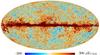
|
|
|
|
|
|
|
|
|
| 143 GHz | 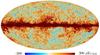
|
|
|
|
|
|
|
|

|
| 217 GHz | 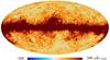
|
|
|
|
|
|
|
|
|
| 353 GHz | 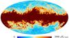
|
|
|
|
|
|
|
|
|
| 545 GHz | 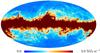
|
. | . | 
|
. | . | 
|
. | . |
| 857 GHz | 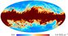
|
. | . | 
|
. | . | 
|
. | . |
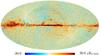
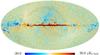
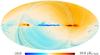
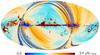
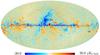
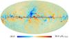
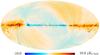
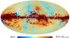
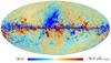
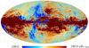
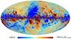
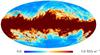
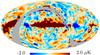
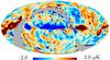
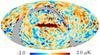
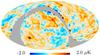
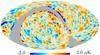
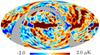
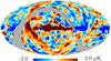
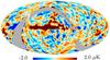
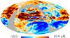
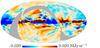
Survey difference maps for the PR2 and the PR3 data
This table shows the PR2 and PR3 survey difference maps ((S1+S3)-(S2+S4))in I, Q, and U. This table is taken from Planck-2020-A3[1] (see detailled explanations there).
| PR2 survey difference maps | PR3 survey difference maps | |||||
|---|---|---|---|---|---|---|
| I | Q | U | I | Q | U | |
| 100 GHz | 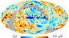
|
|
|
|
|
|
| 143 GHz | 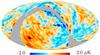
|
|
|
|
|
|
| 217 GHz | 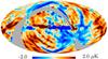
|
|
|
|
|
|
| 353 GHz | 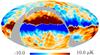
|
|
|
|
|
|
| 545 GHz | 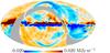
|
. | . | 
|
. | . |
| 857 GHz | 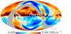
|
. | . | 
|
. | . |
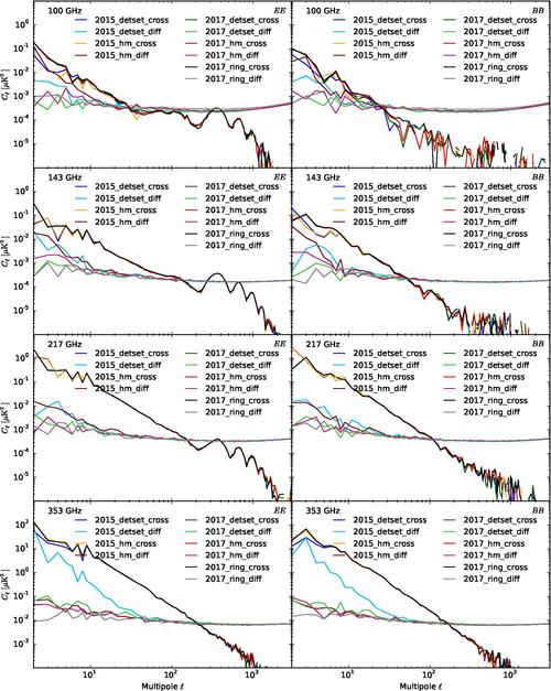
Spectra of the PR2 and the PR3 data splits
This figure shows the EE and BB spectra of the PR2 and PR3 detset, half-mission and rings (for PR3 only) maps at 100, 143, 217, and 353 GHz. The auto-spectra of the difference maps and the cross-spectra between the maps are shown. The sky fraction used here is 43 %. The bins are: bin=1 for ; bin=5 for ; bin=10 for ; bin=20 for ; and bin=100 for . This figure is taken from Planck-2020-A3[1] (see detailled explanations there).
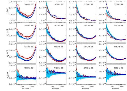
Comparison of the FFP10 simulated noise and systematic residuals and the PR3 data
This figure shows the noise and systematic residuals in TT, EE, BB, and EB spectra, at the three CMB frequencies, for difference maps of the ring (red) and half-mission (blue) null tests binned by . Data spectra are represented by thick lines, and the averages of simulations by thin black lines. For the simulations, we show the 16 % and 84 % quantiles of the distribution with the same colours. This figure is taken from Planck-2020-A3[1] (see detailled explanations there).
References[edit]
- ↑ 1.01.11.21.3 Planck 2018 results. III. High Frequency Instrument data processing and frequency maps, Planck Collaboration, 2020, A&A, 641, A3.
Cosmic Microwave background