CMB spectrum and likelihood code

2015 CMB spectra

General description

TT

The Planck best-fit CMB temperature power spectrum, shown in the figure below, covers the wide range of multipoles [math] \ell [/math] = 2-2508. Over the multipole range [math] \ell [/math] = 2–29, the power spectrum is derived from the Commander: component separation algorithm applied to the combination of Planck 2015 temperature data between 30 and 857 GHz, the 9-year WMAP sky maps, and the 408 MHz Haslam et al. (1982) survey, including 93% of the sky Planck-2015-A10 . The asymmetric error bars associated to this spectrum are the 68% confidence limits and include the uncertainties due to foreground subtraction.

For multipoles equal or greater than [math]\ell=30[/math], instead, the spectrum is derived from the Plik likelihood Planck-2015-A11 by optimally combining the spectra in the frequency range 100-217 GHz, and correcting them for unresolved foregrounds using the best-fit foreground solution from a Planck TT+lowP [math]\Lambda[/math]CDM run. Associated 1-sigma errors include beam uncertainties. Both Commander and Plik are described in more details in the sections below.

File:A15 TT.pdf

TE and EE

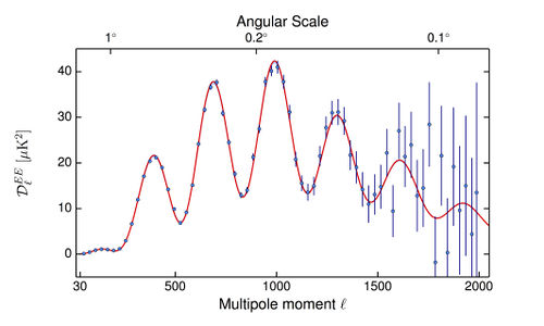
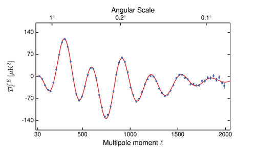
The Planck best-fit CMB polarization and temperature-polarization cross-correlation power spectra, shown in the figure below, cover the multipole range [math] \ell [/math] = 30-1996. The data points relative to the multipole range [math] \ell [/math] = 2-29 will be released in a second moment. Analogously to the TT case, the [math] \ell\ge 30 [/math] spectrum is derived from the Plik likelihood Planck-2015-A11 by optimally combining the spectra in the frequency range 100-217 GHz, and correcting them for unresolved foregrounds using the best-fit foreground solution from a Planck TT,TE,EE+lowP [math]\Lambda[/math]CDM run.

CMB EE spectrum. The red line is the Planck best-fit primordial power spectrum (cf Planck TT+lowP in Table 3 of Planck-2015-A13). The blue shaded area shows the uncertainties due to cosmic variance alone.

CMB TE spectrum. The red line is the Planck best-fit primordial power spectrum (cf Planck TT+lowP in Table 3 of Planck-2015-A13). The blue shaded area shows the uncertainties due to cosmic variance alone.

Production process

The [math]\ell[/math] < 30 part of the Planck TT power spectrum is derived from the Commander approach, which implements Bayesian component separation in pixel space, fitting a parametric model to the data by sampling the posterior distribution for the model parameters Planck-2015-A10. The power spectrum at any multipole [math]\ell[/math] is given as the maximum probability point for the posterior [math]C_\ell[/math] distribution, marginalized over the other multipoles, and the error bars are 68% confidence level; see Planck-2015-A10.

The [math]\ell \ge 30[/math] part of the TT, TE and EE power spectra have been derived by the Plik likelihood, a code that implements a pseudo-Cl based technique, extensively described in Sec. 2 and the Appendix of Planck-2013-XV and Planck-2015-A11. Frequency spectra are computed as cross-spectra between half-mission maps. Mask and multipole range choices for each frequency spectrum are summarized in Section 3.3 of Planck-2015-A13 and in Planck-2015-A11. The final power spectrum is an optimal combination of the 100, 143, 143x217 and 217 GHz spectra, corrected for the best-fit unresolved foregrounds and inter-frequency calibration factors, as derived from the full likelihood analysis (for TT we use the best-fit solutions for the nuisance parameters from the Planck+TT+lowP data combination, while for TE and EE we use the best fit from Planck+TT+lowP, cf Table 3 of Planck-2015-A13). A thorough description of the models of unresolved foregrounds is given in Planck-2015-A11. The spectrum covariance matrix accounts for cosmic variance and noise contributions, together with beam uncertainties. The [math]\ell \ge 30[/math] CMB TT spectrum and associated covariance matrix are available in two formats:

1. Unbinned. TT: 2479 bandpowers ([math]\ell=30-2508[/math]); TE or EE: 1697 bandpowers ([math]\ell=30-1996[/math]).
2. Binned, in bins of [math] \Delta\ell=30 [/math]. TT: 83 bandpowers. TE or EE: 66 bandpowers. We bin the [math] C_\ell [/math] power spectrum with a weight proportional to [math] \ell (\ell+1) [/math], so that the [math] C_{\ell_b} [/math] binned bandpower centered in [math] \ell_b [/math] is: [math] \\ C_{\ell_b}=\Sigma_{\ell \in b} w_{\ell_b\ell} C_\ell \quad \text{with} \quad w_{\ell_b\ell}=\frac{\ell (\ell+1)}{\Sigma_{\ell \in b} \ell (\ell+1)}. \\[/math] Equivalently, using the matrix formalism, we can construct the binning matrix B as: [math]\\ B_{\ell_b \ell}=w_{\ell_b\ell} \\ [/math] where B is a [math] n_b\times n_\ell[/math] matrix, with [math]n_b=83[/math] the number of bins and [math]n_\ell=2479[/math] the number of unbinned multipoles. Thus: [math] \\ \vec{C}_\mathrm{binned}=B \, \vec{C} \\ \mathrm{cov_\mathrm{binned}}= B\, \mathrm{cov}\, B^T \\ \ell_b=B\, \ell \\ [/math] Here, [math] \vec{C}_{binned}\, (\vec{C}) [/math] is the vector containing all the binned (unbinned) [math]C_\ell[/math] bandpowers, [math]\mathrm{cov} [/math] is the covariance matrix and [math]\ell_b[/math] is the weighted average multipole in each bin. Note that following this definition, [math]\ell_b[/math] can be a non-integer. The binned [math]D_{\ell_B}[/math] power spectrum is then calculated as: [math] \\ D_{\ell_b}=\frac{\ell_b (\ell_b+1)}{2\pi} C_{\ell_b} [/math].

Inputs

Low-l spectrum ([math]\ell \lt 30[/math])

• Planck 30 and 44 GHz frequency maps
• Planck 70 to 857 GHz detector and detector set maps
• 9-year WMAP temperature sky maps between 23 and 94 GHz
• 408 MHz survey by Haslam et al. (1982)
• Commander [math]\chi^2[/math] based LM93 confidence mask Planck-2015-A10

High-l spectrum ([math]30 \le \ell \le 2508[/math])

• 100, 143, 143x217 and 217 GHz spectra and their covariance matrix (Sec. 3.3 Planck-2015-A13)
• best-fit foreground templates and inter-frequency calibration factors (Table 3 of Planck-2015-A13)
• Beam transfer function uncertainties Planck-2015-A07

File names and Meta data

The CMB spectrum and its covariance matrix are distributed in a single FITS file named

• COM_PowerSpect_CMB_R2.nn.fits

which contains 7 BINTABLE extensions

1. TT low-ell, unbinned (TTLOLUNB)

with the low ell part of the spectrum, not binned, and for l=2-29. The table columns are

1. ELL (integer): multipole number
2. D_ELL (float): [math]D_ell[/math] as described above
3. ERRUP (float): the upward uncertainty
4. ERRDOWN (float): the downward uncertainty

2. TT high-ell, binned (TTHILBIN)

with the high-ell part of the spectrum, binned into 83 bins covering [math]\langle l \rangle = 47-2499\ [/math] in bins of width [math]l=30[/math] (with the exception of the last bin that is smaller). The table columns are as follows:

1. ELL (integer): mean multipole number of bin
2. L_MIN (integer): lowest multipole of bin
3. L_MAX (integer): highest multipole of bin
4. D_ELL (float): [math]D_\ell[/math] as described above
5. ERR (float): the uncertainty

3. TT high-ell unbinned (TTHILUNB)

with the high-ell part of the spectrum, unbinned, in 2979 bins covering [math]\langle l \rangle = 30-2508\ [/math]. The table columns are as follows:

1. ELL (integer): multipole
2. D_ELL (float): [math]D_\ell[/math] as described above
3. ERR (float): the uncertainty

4. TE high-ell, binned (TEHILBIN)

with the high-ell part of the spectrum, binned into 83 bins covering [math]\langle l \rangle = 47-1988\ [/math] in bins of width [math]l=30[/math] (with the exception of the last bin that is smaller). The table columns are as follows:

1. ELL (integer): mean multipole number of bin
2. L_MIN (integer): lowest multipole of bin
3. L_MAX (integer): highest multipole of bin
4. D_ELL (float): [math]D_\ell[/math] as described above
5. ERR (float): the uncertainty

5. TE high-ell, unbinned (TEHILUNB)

with the high-ell part of the spectrum, unbinned, in 2979 bins covering [math]\langle l \rangle = 30-1996\ [/math]. The table columns are as follows:

1. ELL (integer): multipole
2. D_ELL (float): [math]D_\ell[/math] as described above
3. ERR (float): the uncertainty

6. EE high-ell, binned (EELOLBIN)

with the high-ell part of the spectrum, binned into 83 bins covering [math]\langle l \rangle = 47-1988\ [/math] in bins of width [math]l=30[/math] (with the exception of the last bin that is smaller). The table columns are as follows:

1. ELL (integer): mean multipole number of bin
2. L_MIN (integer): lowest multipole of bin
3. L_MAX (integer): highest multipole of bin
4. D_ELL (float): [math]D_\ell[/math] as described above
5. ERR (float): the uncertainty

7. EE high-ell, unbinned (EEHILUNB)

with the high-ell part of the spectrum, unbinned, in 2979 bins covering [math]\langle l \rangle = 30-1996\ [/math]. The table columns are as follows:

1. ELL (integer): multipole
2. D_ELL (float): [math]D_\ell[/math] as described above
3. ERR (float): the uncertainty

The spectra give [math]D_\ell = \ell(\ell+1)C_\ell / 2\pi [/math] in units of [math]\mu\, K^2[/math]. The covariance matrices of the spectra will be released in a second moment.

Likelihood

The likelihood will soon be released with an accompanying paper and an Explanatory Supplement update.