Appendix of HFI DPC paper

This page is intented to provide complementary figures to those of the 2017 HFI DPC paper (Planck-2020-A3).

---

Section 3.1.2: Very bright regions where the sub-pixel effect in the SRoll CO foreground templates prevent them to be used for cosmology or astrophysics analysis

We simulated the effect to evaluate its level. The difference between the simulated downgraded (at N_side=128) CO simulated maps and the input full resolution (at N_side=2048) CO simulated maps gives the simulated bias introduced by this downgrading for each bolometer. For each frequency channel, these bias maps are converted to HPRs, multiplied by the corresponding CO bandpass coefficients computed by SRoll, and projected onto a frequency map of the bias for the channel. Those frequency averaged bias maps are displayed in the table and given in PLA (LVLV).

For convenience, we also provide the maps of the logarithm of the ratio of the variance, in each N_side=128 pixel, between the bias map and the noise level estimated from the End-to-End simulations. This bias is well determined and specific masks adapted to each scientific analysis can be computed at the appropriate level. Those bias maps are also provided in the PLA.

The table also gives the sky fraction to be masked for thresholding the bias at 100, 10, and 1 % the rms of the bias at N_side=2048 inside the pixel at N_side=128 referred to the rms of the noise at N_side=2048 inside the same pixel at N_side=128.

The effects are largest at 100 GHz. It can also be noted that, for polarization, only less than 10-3 of the sky is affected by this bias at the noise level. For intensity, the biais is an order of magnitude lower. If the user wants to reduce the bias below 10 % of the noise in polarization, 2% of the sky will be affected. Users can also refer to the absolute value of the bias with respect to the CO maps to build the relevant mask.

CO templates

	100 GHz			143 GHz			217 GHz			353 GHz
	I	Q	U	I	Q	U	I	Q	U	I	Q	U
bias maps in muK				.	.	.
bias noise ratio maps				.	.	.
100%	0.01 %	0.01 %	0.07 %	.	.	.	0.00 %	0.01 %	0.01 %	0.00 %	0.01 %	0.01 %
10%	0.55 %	0.97 %	1.80 %	.	.	.	0.04 %	0.29 %	0.19 %	0.01 %	0.38 %	0.29 %
1%	7.39 %	8.63 %	10.81 %	.	.	.	0.90 %	4.98 %	2.79 %	0.46 %	5.81 %	3.38 %

---

Section 5.3.10: for convenience, we reproduce here Figures 6, 7 and 8 of Rosset et al.

This paper is published as Rosset et al. Planck pre-launch status: High Frequency Instrument polarization calibration. 2010b, A&A, 520, A13. () The figures 6, 7 et 8 reproduced hereunder are given in the version on ArXiv 1004.2595

gain errors (1)	polarization efficiency errors (2)	orientation errors (3)
Error creating thumbnail: convert: unable to extend cache `/tmp/magick-30530629UXbMjmuXR': File too large @ error/cache.c/OpenPixelCache/4091.	Error creating thumbnail: convert: unable to extend cache `/tmp/magick-30537_N8AkdHzZC0m': File too large @ error/cache.c/OpenPixelCache/4091.	Error creating thumbnail: convert: unable to extend cache `/tmp/magick-30544c9aDGRerYNNW': File too large @ error/cache.c/OpenPixelCache/4091.

(1) [math]\Delta C_{\ell}[/math] in rms due to gain errors from 0.01% to 1% for E-mode (top) and B-mode (bottom) compared to initial spectrum (solid black lines). Cosmic variance for E-mode is plotted in dashed black line.

(2) [math]\Delta C_{\ell}[/math] in rms due to polarization efficiency errors from 0.1% to 4% for E-mode (top) and B-mode (bottom) compared to initial spectrum (solid black lines). Cosmic variance for E-mode is plotted in dashed black line.

(3) [math]\Delta C_{\ell}[/math] in rms due to various orientation errors from 0.25 to 2 degrees for E-mode (top) and B-mode (bottom) compared to initial spectrum (solid black lines). Cosmic variance for E-mode is plotted in dashed black line.

---

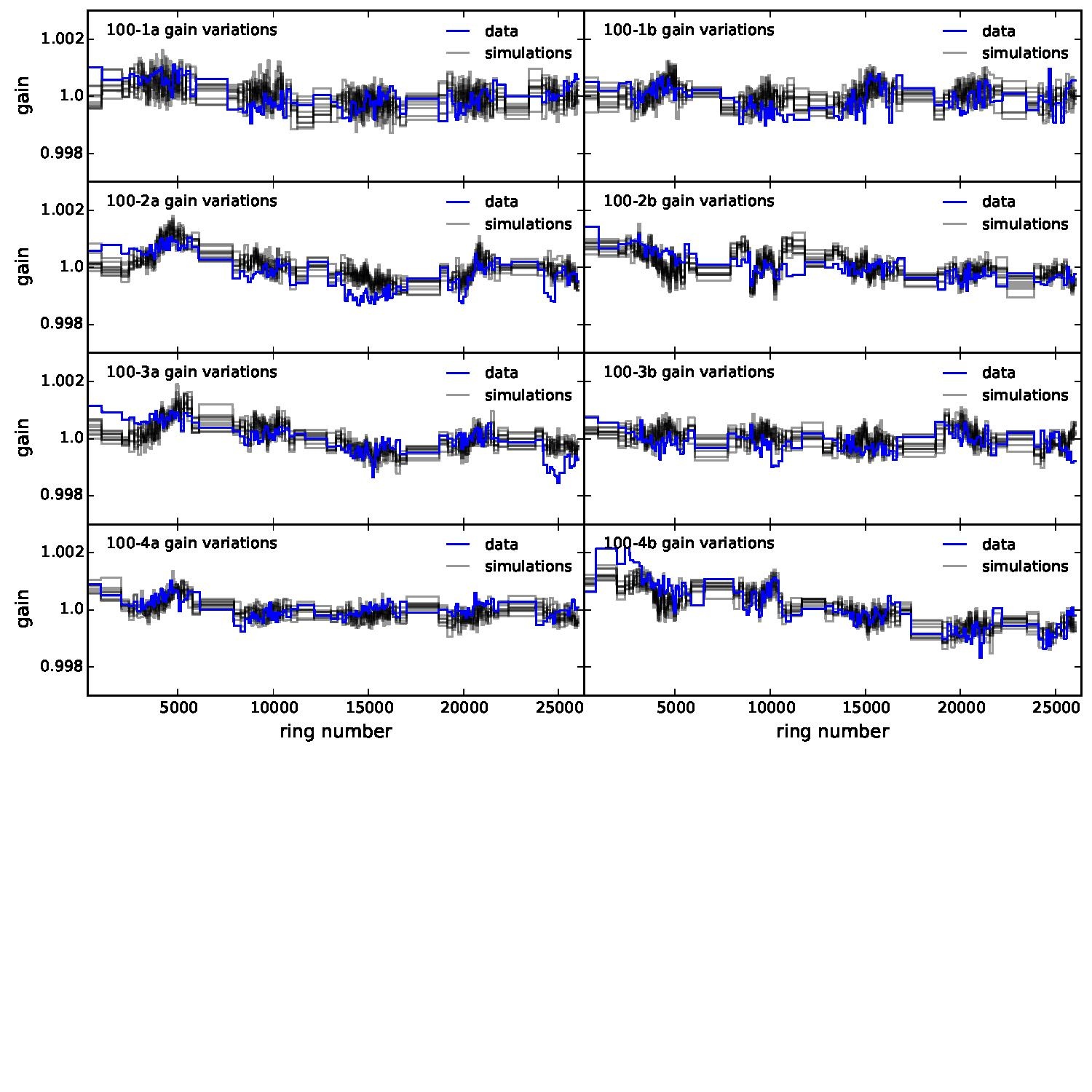
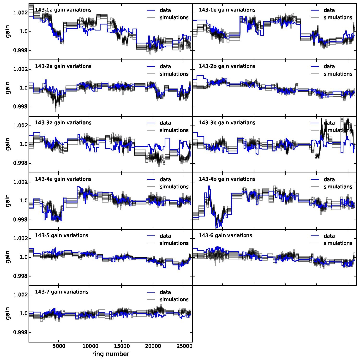
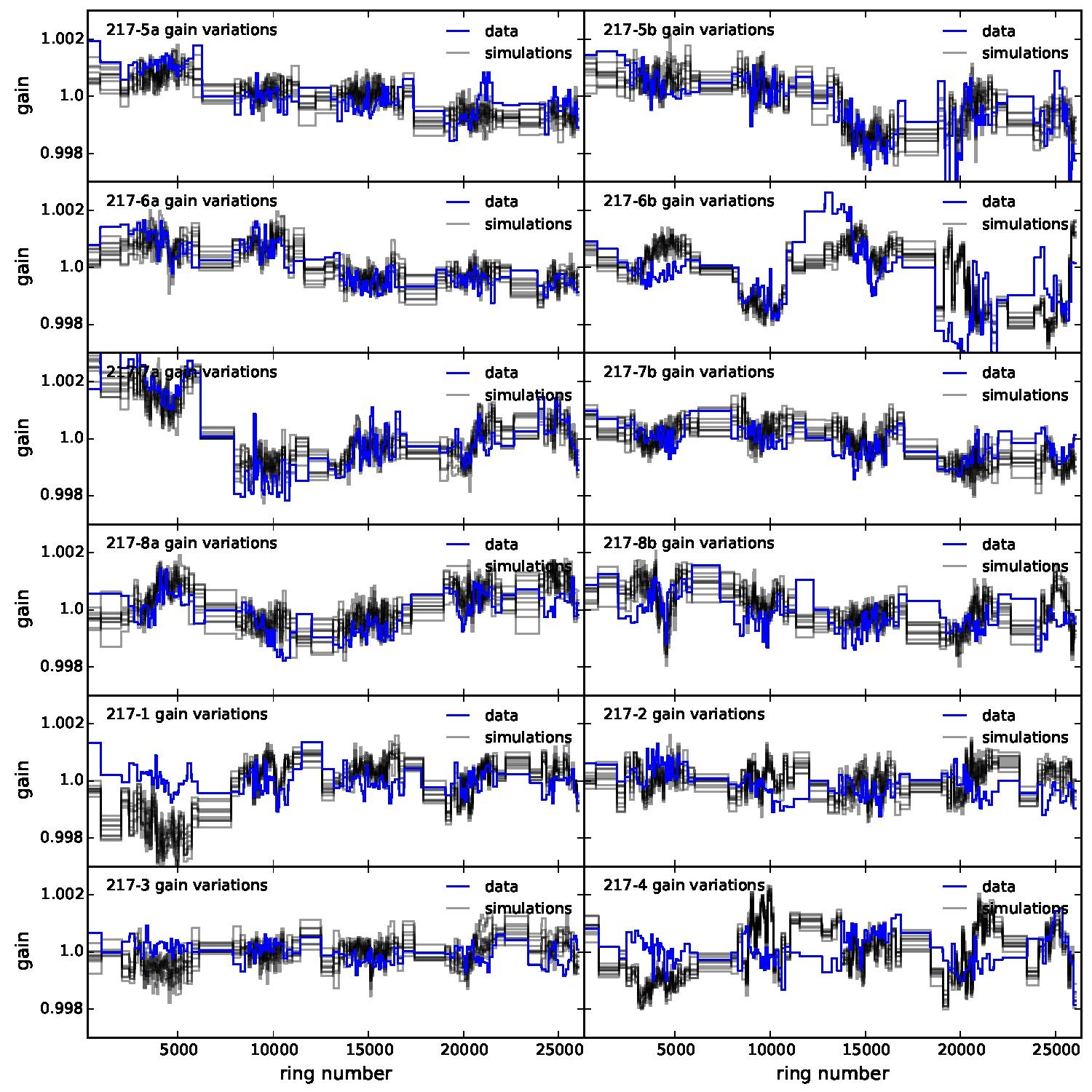
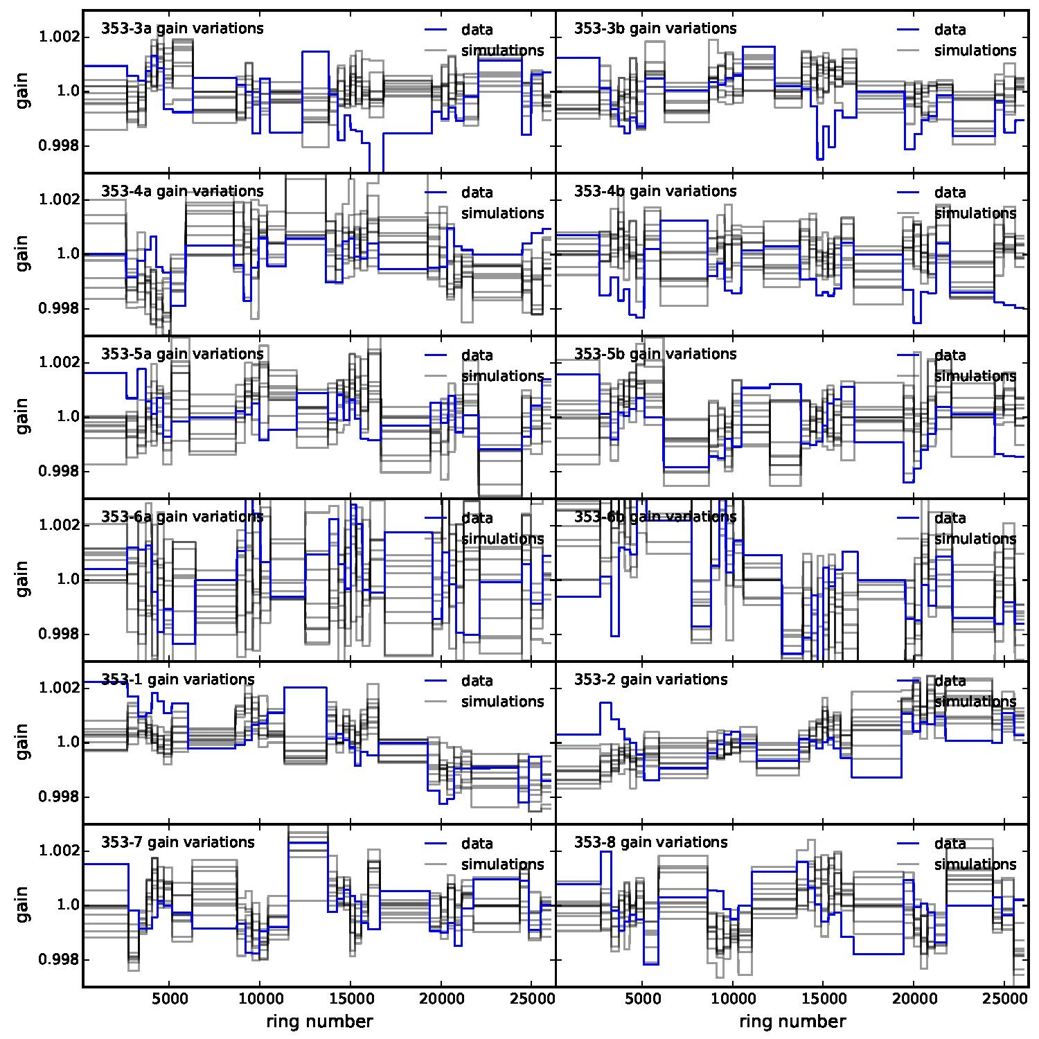
Section 5.5: complementary figures of Fig. 29

Map and power spectra from E2E simulations difference with and without 4K lines.

100 GHz bolometers		143 GHz bolometers		217 GHz bolometers		353 GHz bolometers
100px
.	.
.	.
.	.
.	.	.	.

---

Section 5.13: complementary figures of Fig. 47

ADCNL induced gain time variation as a function of ring numbers. Blue line shows the solved gain variation for the data and grey ones show 10 realizations drawn within the uncertainties of the ADC model.

100 GHz bolometers	143 GHz bolometers	217 GHz bolometers	353 GHz bolometers