Beams

The 2015 Data Release

Introduction

The spatial response reconstruction of the Planck High Frequency Instrument (HFI) is informed by observation of planets. Furthermore, observations of Uranus and Neptune are used to obtain an absolute calibration for the 545 and 857 GHz channels.

The spatial response, also known as the beam response or the point spread function, relates the absolute calibration to different angular scales.

All content found on this page, as well as further information regarding the beam products used for the 2015 release of Planck data, can be found in the HFI DPC Paper 1 .

Planet and main beam description

We follow the nomenclature of Planck Collaboration VII Planck-2013-VII (2014), where the scanning beam is defined as the coupled response of the optical system, the deconvolved time response function, and the software lo-wpass filter applied to the data. The effective beam represents the averaging of signal due to the scanning of the telescope and mapmaking, and varies from pixel to pixel across the sky.

Here we redefine the main beam to be the scanning beam out to 100 arcmin from the beam axis. The sidelobe structure at this radius is dominated by diffraction at the mirror edges and falls as ([math]\propto \theta ^{-3}[/math]) where [math]\theta[/math] is the angle to the main beam axis. The main beam is used to compute the effective beam and the effective beam window function, which describes the filtering of sky signals. The smearing of the main beam cannot be significantly reduced without boosting the high-frequency noise. The regularization function (a low-pass filter) chosen has approximately the same width as the instrumental transfer function. The deconvolution significantly reduces the long tail of the scanning beam (see Fig. 1). The deconvolution also produces a more symmetric time response, so residual “streaking” appears both ahead and behind the main beam, though ahead of the beam it is at a level of less than 1E−4 of the peak response. The far sidelobes are defined as the response from [math]\theta[/math] > 5 deg, roughly the minimum in the optical response. The response begins to rise as a function of angle [math]\theta[/math] beyond this due to spillover. The far sidelobes are handled separately from the beam effects (see Sect. 4.6 for justification and Paper 2 for details).

Figure 1: A scan across Jupiter with bolometer 143-1b, pre-deconvolution in black, post-deconvolution in red. The plotted y-axis range is linear within the range [math]\pm 10^{-6}[/math] and logarithmic elsewhere. Similarly, the x-axis range is linear within the range [math]\pm 0.16[/math] s, and logarithmic outside

Key Changes

There are several key changes in the reconstruction of the main beam since the 2013 data release, these include:

• The time ordered data from Saturn and Jupiter observations are merged prior to B-spline decomposition, accounting for residual pointing errors and variable seasonal brightness. This is achieved by determining a scaling factor and a pointing offset by fitting the time ordered data to a template from a previous estimate of the scanning beams. We iterate the planet data treatment updating the template with the reconstructed scanning beam. The process converges in five iterations within a tenth of a percent accuracy in the effective beam window function.
• Steep gradients in the signal close to the planet reduce the completeness of the standard glitch detection and subtraction procedure; therefore the planet timelines are deglitched a second time.
• The beam pipeline destripes the planet data, estimating a single baseline between 3 and 5 deg before the peak for each scanning circle. Baseline values are smoothed with a 40 circles sliding window. The entire scanning circle is removed from the beam reconstruction if the statistic in the timeline region used to estimate the baseline is far from Gaussian.
• The main beam is now recontructed on a square grid that extends to a radius of 100 arcmin from the centroid, as opposed to 40 arcmin in the 2013 data release. The cutoff of 100 arcmin was chosen such that a diffraction model of the beam at large angles from the centroid predicts that less than 5E-5 of the total solid angle is missing.
• The scanning beam is constructed by combining data from Saturn observations, Jupiter observations, and physical optics models using GRASP software.
• No apodization is applied to the scanning beam map.

The update of the time response deconvolved data has slightly changed the scanning beam, the effective beam solid angles and the effective beam window functions.

Table 1. Band-average scanning beam solid angle ([math]\Omega _\mathrm{SB} [/math]) and Monte Carlo-derived errors ([math]\Delta\Omega _\mathrm{MC}[/math]) including noise, residual glitches, and pointing uncertainty.

Band	[math]\Omega _\mathrm{SB}[/math]	[math]\Delta \Omega _\mathrm{MC}[/math]
[GHz]	[arcmin[math]^2[/math]
100	104.62	0.13 %
143	58.50	0.07 %
217	26.92	0.13 %
353	25.93	0.09 %
545	25.23	0.08 %
857	23.04	0.08 %

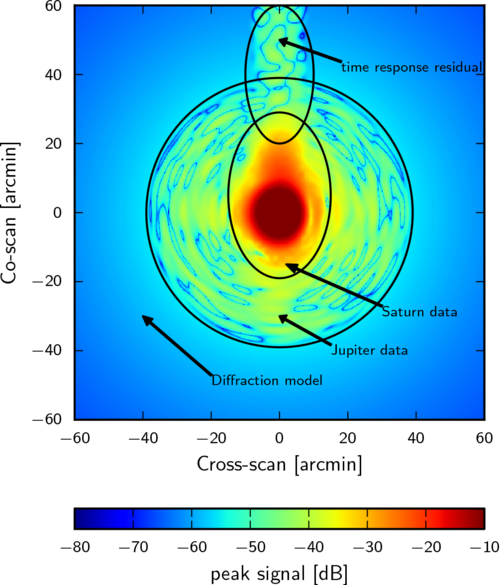
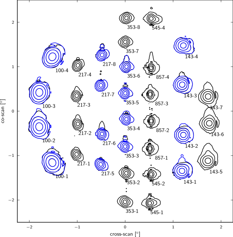
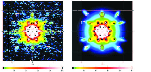
A portion of the near sidelobes was not accounted for in the effective beam window function of the 2013 data (see Planck-2013-VI). To remedy this, the domain of the main beam reconstruction is extended to 100 arcmin, with no apodization. Saturn data are used where they are signal-dominated. Where the signal-to-noise ratio of the Saturn data fall below 9, azimuthally binned Jupiter data are used. At larger angles, below the noise floor of the Jupiter data, we use a power law ([math]\propto\theta^{-3}[/math]) whose exponent is derived from GRASP to extend the beam model to 100 arcmin. Figure Fig. 2 shows a scanning beam map diagram of the regions handled differently in the hybrid beam model. A summary of the solid angles of the hybrid beams is shown in Table 1. Figure 3 shows a contour plot of all the scanning beams referenced to the center of the focal plane.

Figure 2: Scanning beam map for detector 143-6 showing a rough diagram of the regions that are handled with a different data selection or binning.

Figure 3: B-spline hybrid scanning beams reconstructed from Mars, Saturn, and Jupiter. The beams are plotted in logarithmic contours of −3, −10, −20, and −30 dB from the peak. PSB pairs are indicated with the a bolometer in black and the b bolometer in blue.

Beam Error Budget

As in the 2013 release, the beam error budget is based on an eigenmode decomposition of the scatter in simulated planet observations. A reconstruction bias is estimated from the ensemble average of the simulations. We generate 100 simulations for each planet observation that include pointing uncertainty, cosmic ray glitches, and the measured noise spectrum. Simulated glitches are injected into the timeline with the correct energy spectrum and rate ({{PlanckPapers|planck2013-p03e}) and are detected and removed using the deglitch algorithm. Noise realizations are derived as shown in Sect. 5.3.1. Pointing uncertainty is simulated by randomizing the pointing by 1.5 arcsec rms in each direction. The improved signal-to-noise ratio compared to 2013 leads to smaller error bars: for instance, at [math]\ell[/math] = 1000 the uncertainties on [math]B_\ell^2[/math] are now (2.2, 0.84, 0.81)× E-4 for 100, 143, and 217 GHz frequency-averaged maps respectively, reduced from the previous uncertainties of (61, 23, 20)× E−4.

A “Reduced Instrument Model” (RIMO; see The_RIMO) containing the effective [math]B(\ell)[/math] for temperature and polarization detector sets, for auto- and cross-spectra, at 100 to 217 GHz is included in the release, for a sky fraction of 100 %. Another RIMO is provided for a sky fraction of 75 %. They both contain the first five beam error eigenmodes and their covariance matrix, for the multipole ranges [0, [math]\ell_{\mathrm{max}}[/math]] with [math]\ell_{\mathrm{max}}[/math] = 2000, 3000, 3000 at 100, 143, and 217 GHz respectively (instead of 2500, 3000, 4000 previously). These new ranges bracket more closely the ones expected to be used in the likelihood analyses, and ensure a better determination of the leading modes on the customized ranges. As described in Appendix A7 of Planck Collaboration XV (2014) Planck-2013-XV, these beam window function uncertainty eigenmodes are used to build the [math]C_{\ell}[/math] covariance matrix used in the high-[math]\ell[/math] angular power spectrum likelihood analysis. It was found that the beam errors are negligible compared to the other sources of uncertainty and have no noticeable impact on the values or associated errors of the cosmological parameters.

Consistency of Beam Reconstruction

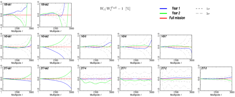
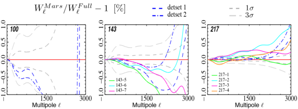
To evaluate the accuracy and consistency of the beam reconstruction method, we have compared beams reconstructed using Mars for the main beam part instead of Saturn, and using data from Year 1 or Year 2 only. We compared the window functions obtained with these new beams to the reference ones; new Monte Carlo simulations were created to evaluate the corresponding error bars, and the results are shown in Figs. 4 and 5. Note that the effective beam window functions shown in these figures are not exactly weighted for the scan strategy, rather we plot them in the raster scan limit where B2 is defined as the sum over [math]m[/math] the [math]B_\ell^m[/math]. The eigenmodes were evaluated for these different data sets allowing us to compare them with the reference beam by a [math]\chi ^2[/math] analysis. The discrepancy between each data set and the reference beam is fitted using “dof”=5 eigenmodes using [math]\ell _\mathrm{max}[/math] = 1200, 2000, 2500 for 100, 143 and 217 channels respectively. The [math]\chi ^2[/math] is then defined as:

[math] \chi^2 = \sum_{i=1}^{\mathrm{dof}} (c_i / \lambda_i)^2 \label{eq:chi2} [/math]

where [math]c_i[/math] is the fit coefficient for eigenvector i, with eigenvalue [math]\lambda _i [/math]. For each data set, the [math]p[/math]-value to exceed this [math]\chi ^2[/math] value for a [math] \chi ^2[/math] distribution with dof degrees of freedom is indicated in Table 2. A high [math]p[/math]-value indicates that the given data set is consistent with the reference beam within the simulation-determined error eigenvectors, with 100 % indicating perfect agreement. We find excellent agreement between the yearly and nominal beams for the SWB bolometer channels. However, in order to obtain reasonable beam agreement for the PSB detector sets, we find that the yearly beam errors must be scaled by a factor 4 to achieve agreement. We conclude that there is an unknown systematic error in the beam reconstruction that is not accounted in the simulations used to estimate the beams accounting in the Monte Carlo error bars. We assign a scaling factor 4 to the error eigenmodes to account for this systematic error. The additional error scaling has a negligible effect on the cosmological parameters.

Figure 4: Comparison of Year 1 and Year 2 based beams with the reference beam (Full Mission). Window functions are calculated using Quickbeam in raster scan configuration. Error bars are computed using MC simulations for Year 1 and Year 2, taking the maximal one for each.

Figure 5: Comparison of Mars-based beams with the reference beam (Full Mission). Mars-based beams are constructed from Mars data for the main beam ([math]\lesssim [/math] 10 arcmin) and Saturn and Jupiter data for the larger scales. Window functions are calculated using Quickbeam in raster scan configuration. Error bars are computed using MC simulations for Mars.

Table 2. [math]P[/math]-values in percent for the [math]\chi ^2[/math] comparison of the nominal beam with Year 1 and Year 2 data sets, following the definition in above equation.

Band	Year 1	Year 2
100-ds1	66.95	92.44
100-ds2	85.12	75.99
143-ds1	72.24	99.83
143-ds2	1.14	16.81
143-5	94.88	97.57
143-6	96.14	98.78
143-7	93.78	95.67
217-ds1	78.12	69.74
217-ds2	27.33	30.87
217-4	95.99	68.44
217-1	99.08	97.49
217-2	97.18	98.86
217-3	97.59	99.07

Colour Correction of the Beam Shape

In general, the measured beam shape is a function of the spectral energy distribution (SED) of the measurement source. This is of particular concern because we measure the beam on a source with a roughly Rayleigh-Jeans SED, yet we use the effective beam window function to correct the CMB.

Planck Collaboration VII (2014) Planck-2013-VII described possible levels of this bias using GRASP calculations with the pre-launch telescope model (Maffei et al. 2010 ; Tauber et al. 2010 ). The prelaunch calculations did not agree well enough with the data to allow a direct application of the colour correction. A new telescope model based on flight data, and presented in a forthcoming paper, predicts beams that agree better with the data at 100–217 GHz, but show a worse agreement at 353 GHz. The new model predicts a different beam shape colour correction though at a similar order of magnitude to that shown in Planck Collaboration VII (2014) Planck-2013-VII. This work is ongoing and will be completed after the 2015 release.

We search for a possible signature of the colour correction effect in the data. First, we check for consistency in the CMB angular power spectra derived from different detectors and frequency bands using the SMICA algorithm, in order to find discrepancies in beam shape and relative calibration of different data subsets on the CMB (Planck Collaboration A13 2014 Planck-2015-A11). There are hints of differences that are orthogonal to the beam error eigenmodes and appear as changes in relative calibration, but the preferred changes are at the 0.1 % level. Because this correction is of the same order of magnitude as the relative calibration uncertainty between detectors, we treat it as insignificant.

Second, we look at the relative calibration between detectors within a band on compact sources as a function of the source SED. In this method, any discrepancies due to solid angle variation with SED are degenerate with an error in the underlying bandpass. Additionally, because of the lack of bright, compact sources with red spectra, this method is limited in its signal-to-noise ratio. In the limit that any detected discrepancy is completely due to solid-angle variation with colour, at the level of 1 % in solid angle we do not detect variations consistent with the physical optics predictions. Given the lack of measurement of this effect at the current levels of uncertainty, as well as uncertainties in modelling of the telescope, we note that this effect may be present at a small level in the data, but do not attempt to correct for it or include it in the error budget.

Data Products

Beam products are available from the instrument model (The_RIMO) and further described in Scanning_Beams and Effective_Beams

The 2013 Data Release

Scanning Beams

The scanning beams describe the instrument’s instantaneous beam profile. Due to the near constant spin rate of the spacecraft, time domain effects (including residual time response and lowpass filtering) are degenerate with the spatial response due to the optical system. The scanning beam reconstruction recovers both of these effects, aside from residual time domain effects on a longer time scale than can be captured with the extent of the scanning beam model.

In Planck-2013-VII we consider two models of the beam in order to better understand systematics in the reconstruction. Here we describe only the B-Spline beams which are used to compute the delivered effective beam (see next section).

B-Spline Beam construction

We use seasons 1 and 2 of the Mars observation to reconstruct the beam. The data are processed with the bigPlanets TOI processing (see here or Section 3.11 of Planck-2013-VI for more info). We use JPL Horizons ephemerides to determine the pointing of each detector relative to the planet. We subtract the astrophysical background in the time domain using a bicubic interpolation of the Planck maps.

The time ordered data are used to fit a two dimensional B-Spline surface using a least square minimization and a smoothing criterion to minimize the effects of high spatial frequency variations. We therefore assume the scanning beam to be smooth. The smoothing criterion as well as the locations of the nodes used to compute the B-Spline basis functions are set using GRASP physical optics simulations as inputs which are the best assumptions on the spatial frequency content of the in-flight beams.

The smoothing criterion is defined as follows:

[math]\eta = \displaystyle{\sum_{i=1}^{g}\left(b^{k}(\lambda_{i+})-b^{k}(\lambda_{i-})\right)^2} \label{smoothcrit}[/math]

[math]\begin{aligned} \eta &: \mbox{ Smoothing Criterion}\\ b^k &: \mbox{ $k^{th}$ beam derivative evaluated on the nodes locations}\end{aligned}[/math]

And the global inversion criterion :

[math]\zeta = \eta + p\times \delta[/math]

with [math]\delta[/math] usual least square estimator and [math]p[/math] coefficient giving the relative weight to [math]\delta[/math] with respect to the smoothing criterion.

[math]\delta = \displaystyle{\sum_{r=1}^{m}}\left(y_{r} - b(x_{r})\right)^2\label{estimator}[/math]

[math]\begin{aligned} \delta &: \mbox{ usual least square criterion}\\ r &: \mbox{ indice relative to the m data points, } r \in \{1, \ldots, m\}\\ y_r &: \mbox{ planet data of sample r}\\ x_r &: \mbox{ pointing of sample r}\\ b &: \mbox{ reconstructed beam}\end{aligned}[/math]

The B-Spline nodes are located on a regular spaced grid in the detector coordinate framset. At the edge of the reconstructed beam map area, 4 coincident nodes are added to avoid vanishing basis functions.

Let [math]B_{i, k+1}[/math], [math]k[/math] degree B-Spline build using nodes {[math]\lambda_{i}, ..., \lambda_{i+k+1}[/math]} (De Boor & Cox, 1972) :

[math]B_{i,1}(x) = \left\{ \begin{array}{l} 1, \mbox{ si } x \in \mbox{[} \lambda_{i}, \lambda_{i+1} \mbox{[}\\ 0, \mbox{ si } x \notin \mbox{[} \lambda_{i}, \lambda_{i+1} \mbox{[} \end{array} \right.[/math]

[math]B_{i, l+1}(x) = \displaystyle{\frac{x - \lambda_{i}}{\lambda_{i+l} - \lambda_{i}}} B_{i,l}(x) + \displaystyle{\frac{\lambda_{i+l+1}-x}{\lambda_{i+l+1}-\lambda_{i+1}}} B_{i+1, l}(x)[/math]

[math]l=1, \ldots, k[/math]

Figure 1: Focal plane plot of B-Spline scanning beams using in-flight pointing reconstruction. The contours are -3,-10,-20,-30 dB from the peak, and for PSB pairs the "a" bolometer is plotted in black and "b" in blue.

Simulations and errors

We estimate the reconstruction bias and noise in the measurements using an ensemble of simulated planet observations for each channel. Further details are discussed in Planck-2013-VII. Kept fixed in each simulation are:

• the input beam assumed: we use a supersampled version of the reconstructed B-Spline beam (or whatever comes out of the current ongoing tests!)
• Astrophyical background is the same as that subtracted from the real data.
• StarTracker pointing (using the ptcor6 pointing model).

The following are varied in each simulation:

• detector noise realizations obtained by filtering randomly generated white noise with the measured noise PSDs
• random pointing errors with 2" rms, and a spectrum that replicates the real errors.
• simulated glitches and the deglitching procedure
• Mars brightness temperature variability

400 simulated timelines are generated for each bolometer and for each of the two seasons of Mars observations used in the beam reconstruction. The simulated timelines are made into beam maps, projecting onto the B-Spline basis in the same way as the real data.

The beam maps are propagated to effective beam window functions using the QuickBeam approach (see effective beams below) and used to evaluate the reconstruction bias and to construct error eigenmodes in the effective beam window function.

Residuals

There are two known beam effects that are not included in the main beam model and are estimated as a separate bias in flux and angular power spectrum measurement: 1. long tails due to errors in low frequency time response deconvolution, and 2. near sidelobes.

We stack all five observations of Jupiter to estimate the long time scale residuals due to incomplete deconvolution of the long time scale response.

Effect of Mirror Support Print-through

The Planck reflectors suffer from print-through of the honeycomb structures that support the carbon-fibre face sheets. While the size of the deformation has been measured during tests below room temperature to be less than 20 microns, it is the strict periodicity of the deformation that contributes most to the additional beam-shape contribution. A simple grating equation has been shown to describe the angular positions of the resulting near side lobes very well:

[math] \displaystyle{ \sin \theta _n = \frac{n \lambda}{Yd} } \label{DimplingLobes}[/math]

• [math]\theta _n [/math]: the angular position of the n'th order lobe from the central beam peak
• [math]\lambda [/math]: the wavelength of the radiation
• [math]d [/math]: the grating spacing of the periodicity
• [math]Y [/math]: factor that describes the position of the each reflector along the optical path
• [math]Y=1.00 [/math]: for the primary reflector
• [math]Y=1.80 [/math]: for the secondary reflector

Three possible periodicities (19.6mm, 30mm, 52mm) in the honeycomb array dominate the Planck dimpling pattern for the 857 GHz detectors, though only those for the 52mm periodicity can be seen for the 545 GHz and 353 GHz detectors. For the highest frequency detectors, only the weaker lobes due to the 19.6mm and 30mm periodicities are seen outside the 40 arcminute beam window, but they contribute at most (0.05 ± 0.008)% to the integrated beam.

A map of Jupiter has been created for each 857 GHz detector, using the first four surveys, with the background subtracted using the same sky area for the survey taken 12 months before in which the planet is not present. The background-subtracted maps for each survey were then stacked to make a single map for each of the four detectors and these were further stacked to create a single 857 GHz band map, using the standard detector weightings proportional to 1/(NET)². All the maps have 96 pixels per side, covering ±1.4º, and are scaled to the RMS noise of the background. Central beam values range from 205,000 to 256,000, depending on the noise of the detector.

For each of these five maps of Jupiter an elliptical gaussian main beam has been fitted, and the amount of saturation estimated by finding the peak increase that gives the best gaussian fit, typically 10--20%. A circular ruze envelope was also fitted together with a tilted gaussian component slightly offset from the beam in the cross-scan (optical X axis) direction, using data more than 0.13º from the beam, with the known positions of the dimpling lobes masked out. Once these strongest components were removed, a tilted elliptical gaussian was fitted for each visible dimpling lobe in up to 5 different sets of lobes, however the innermost lobe set (52mm periodicity) is generally obscured by the ruze component and for the outermost set (19.6mm periodicity) most lobes are too weak to be fitted for individual detectors. The contributing areas of the lobes were determined by three methods: from the fitted gaussians; from summation within boxed areas using offsets determined from surrounding boxed areas; from summation in the boxed areas using an offset determined from gaussian fitting.

The uncertainties in the beam component areas given here include the spread in values from these different methods. Similarly, the lobe peaks in decibels are calculated using the raw, fitted and estimated desaturated beam peak values, and the uncertainties reflect the variations produced by the three methods. Averaged over the five map fittings, the dimpling lobes contribute (0.47 ± 0.13)% of the beam area, while the ruze envelope accounts for (9.2 ± 0.7)% of the beam with the main beam making up the remaining (90.3 ± 0.7)%.

For lower frequencies the dimpling lobes are less visible and will not be discussed here. For example, the noise floor for the 545 GHz band map is about 47 dB below the observed Jupiter peak, so that no dimpling lobes are visible further out than the 52mm lobes at 0.61º. For 353 GHz the noise floor is at about 38 dB so that even the 52mm lobes are not observed.

Figure 2: Stacked Jupiter map for the 857 GHz detectors. Left: the data with main beam and ruze envelope subtracted. Right: the fitted elliptical gaussian dimpling lobes with GRASP contours plotted on top.

This figure shows how the dimpling lobes seen for the 857GHz band Jupiter map correspond to the contours calculated by the physical optics GRASP package, produced by TICRA, Denmark. The GRASP simulation was performed for the 857-1 detector and assumed a uniform dimpling distortion of 10 microns. The biggest departure from the simple grating model, is that the lobe pattern is elongated in the cross-scan (vertical) direction---lobes that should lie on a line 30º from the vertical are consistently found around 25º and those on the 60º line cluster around 53º. This is due to the offset geometry of the mirror system, whereby the dimpling print-though is foreshortened along the optical x-axis due to the tilt of the mirrors, producing greater lobe spacing as seen by the incoming photons. The amplitudes of the fitted dimpling lobes vary significantly within each set whereas the GRASP model shows a constant amplitude for lobes within a set, except for the 30mm periodicity. Similar amplitudes are seen in lobes lying directly across the beam centre from each other, indicating that facesheet dimpling has not occurred uniformly in all directions as the GRASP model assumes.

For the 30mm periodicity the vertical lobes are significantly weaker than those at the sides just as the GRASP model also shows. Generally, the fitted lobes are somewhat stronger than those seen by GRASP, indicating that the dimpling is indeed larger than 10 microns. While the dimpling lobes are measureable at the highest two frequencies, with a strong source (i.e. Jupiter), 90% of the dimpling lobe area at 857GHz, and 10% for all other frequencies, already appears in the beam functions described above and need no further correction. However, the presence of the uniform dimpling lobes provides a useful window by which to investigate the mirror geometry.

Effective Beams

The effective beam is the average of all scanning beams pointing at a certain direction within a given pixel of the sky map for a given scan strategy. It takes into account the coupling between azimuthal asymmetry of the beam and the uneven distribution of scanning angles across the sky. It captures the complete information about the difference between the true and observed image of the sky. They are, by definition, the objects whose convolution with the true CMB sky produce the observed sky map.

Several methods of effective beams determination have been developped and cross-validated. The main products are produced using FEBeCoP and details of the processing are given in the Effective Beams products page. See also the equivalent page discussing the LFI beams

FEBeCoP

---

The full algebra for this method for the calculation of effective beams was presented in . Here we summarise the main results. The observed temperature sky [math]\widetilde{\mathbf{T}} [/math] is a convolution of the true sky [math]\mathbf{T} [/math] and the effective beam [math]\mathbf{B}[/math]:

[math] \widetilde{\mathbf{T}} \ = \ \Delta\Omega \, \mathbf{B} \cdot \mathbf{T}, \label{eq:a0} [/math]

where

[math] B_{ij} \ = \ \left( \sum_t A_{ti} \, b(\hat{\mathbf{r}}_j, \hat{\mathbf{p}}_t) \right) / \left({\sum_t A_{ti}} \right) \, , \label{eq:EBT2} [/math]

[math]t[/math] is time samples, [math]A_{ti}[/math] is [math]1[/math] if the pointing direction falls in pixel number [math]i[/math], else it is [math]0[/math], [math]\mathbf{p}_t[/math] represents the exact pointing direction (not approximated by the pixel centre location), and [math]\hat{\mathbf{r}}_j[/math] is the centre of the pixel number [math]j[/math], where the scanbeam [math]b(\hat{\mathbf{r}}_j, \hat{\mathbf{p}}_t)[/math] is being evaluated (if the pointing direction falls within the cut-off radius of [math]\sim 2.5 \times[/math] FWHM.

The algebra is a bit more involved for polarised detectors. The observed stokes parameters at a pixel [math]i[/math], [math](\widetilde{I}, \widetilde{Q}, \widetilde{U})_i[/math], are related to the true stokes parameters [math](I, Q, U)_i[/math], by the following relation:

[math] ( \widetilde{I} \quad \widetilde{Q} \quad \widetilde{U})_i^T \ = \ \Delta\Omega \sum_j \mathbf{B}_{ij} \cdot (I \quad Q \quad U)_j^T, \label{eq:a1} [/math]

where the polarised effective beam matrix

[math] \mathbf{B}_{ij} \ = \ \left[ \sum_t A_{tp} \mathbf{w}_t \mathbf{w}^T_t \right]^{-1} \sum_t A_{ti} \, b(\hat{\mathbf{r}}_j, \hat{\mathbf{p}}_t) \, \mathbf{w}_t \mathbf{W}^T(\hat{\mathbf{n}}_j,\hat{\mathbf{p}}_t) \, , \label{eq:a2} [/math]

and [math]\mathbf{w}_t [/math]and [math]\mathbf{W}(\hat{\mathbf{r}}_j, \hat{\mathbf{p}}_t) [/math] are the the polarisation weight vectors, as defined in .

The task is to compute [math]B_{ij}[/math] for temperature only beams and the [math]3 \times 3[/math] matrices [math]\mathbf{B}_{ij}[/math] for each pixel [math]i[/math], at every neighbouring pixel [math]j[/math] that fall within the cut-off radius around the the center of the [math]i^\text{th}[/math] pixel.

The effective beam is computed by stacking within a small field around each pixel of the HEALPix sky map. Due to the particular features of Planck scanning strategy coupled to the beam asymmetries in the focal plane, and data processing of the bolometer and radiometer TOIs, the resulting Planck effective beams vary over the sky.

FEBeCoP, given information on Planck scanning beams and detector pointing during a mission period of interest, provides the pixelized stamps of both the Effective Beam, EB, and the Point Spread Function, PSF, at all positions of the HEALPix-formatted map pixel centres.

FICSBell

For more details, see Planck-2013-VII.

Since the HFI beams are not azimuthally symmetric, the scanning strategy has to be taken into account in the effective beam response modelling. This is done using the FICSBell method (Hivon et al, in preparation), which generalizes to polarization and to include other sources of systematics the approach used for TT [math]C(l)[/math] estimation in WMAP-3yr and by Smith et al (2007) in the detection of CMB lensing in WMAP maps. The different steps of the method used for this study can be summarized as follows:

1. The scanning related information (i.e., statistics of the orientation of each detector within each pixel) is computed first, and only once for a given observation campaign:

   [math] w^d_s({\bf r}_p) = \sum_j e^{i s \psi_j}, \label{eq:e1} [/math]

   where [math]\psi_j[/math] is the orientation of the detector with respect to the local meridian during the measurement [math]j[/math] occurring in the direction [math]{\bf r}_p[/math]. Note that the [math]s=0[/math] moment is simply the hit count map. The orientation hit moments are computed up to degree [math]s=6[/math]. At the same time, the first two moments of the distribution of samples within each pixel (i.e., the centre of mass and moments of inertia) are computed and stored on disc.

2. The scanning beam map or beam model of each detector [math]d[/math] is analyzed into its Spherical Harmonics coefficients

   [math] b^d_{ls} = \int d{\bf r} B_d({\bf r}) Y_{ls}({\bf r})\label{scanningBlm} [/math]

   where [math]B_d(\bf{r})[/math] is the beam map centered on the North pole, and [math]Y_{ls}(\bf{r})[/math] is the Spherical Harmonics basis function. Higher [math]s[/math] indexes describes higher degrees of departure from azimuthal symmetry and, for HFI beams, the coefficients [math]b^d_{ls}[/math] are decreasing functions of [math]s[/math] at most multipoles considered. It also appears that, for [math]l\lt 3000[/math] (or [math]l\lt 2000[/math] at 100GHz), the coefficients with [math]|s| \gt 6[/math] account for much less of [math]0.1\%[/math] of the beam solid angle. For these reasons, only modes with [math]|s| \le 6[/math] are considered in the present analysis. Note that in the 2013 analysis, where the scanning beams were slightly less elongated because of different transfer functions deconvolution, the analysis was performed with modes [math]|s| \le 4[/math].

3. For a given CMB sky realization [math]t[/math], described by its spherical harmonics coefficients [math]a_{\ell m} = \int d{\bf r} t({\bf r}) Y_{\ell m}({\bf r})[/math], the [math]b^d_{\ell s}[/math] coefficients computed above are used to generate [math]s[/math]-spin weighted maps,

   [math] m^d_{s}({\bf r}) = \sum_{\ell m} b^d_{\ell s}\ a_{\ell m}\ {}_sY_{\ell m}({\bf r}), \label{eq:e3} [/math]

   as well as the first and second derivatives, using standard HEALPix tools.

4. The spin weighted maps and orientation hit moments of the same order [math]s[/math] are combined for all detectors involved, to provide an “observed” map

   [math] m({\bf r}) = \left(\sum_d \sum_s w^d_s({\bf r}) m^d_s({\bf r})\right) / \sum_d w^d_0({\bf r}). \label{eq:e4} [/math]

   Similarly the local spatial derivatives are combined with the location hit moments to describe the effect of the non-ideal sampling of each pixel (see Pixelization Artifacts section). In this combination, the respective number of hits of each detector in each pixel is considered, as well as the weighting (generally proportional to the inverse noise variance) applied to each detector in order to minimize the final noise.

5. The power spectrum of this map can then be computed, and compared to the input CMB power spectrum to estimate the effective beam window function over the whole sky, or over a given region of the sky.

Monte-Carlo (MC) simulations in which the sky realizations are changed can be performed by repeating steps 3, 4 and 5. The impact of beam model uncertainties can be studied by including step 2 into the MC simulations.

QuickBeam

For more details, see Planck-2013-VII

Formalism

Planck observes the sky after convolution with a “scanning beam”, which captures its effective response to the sky as a function of displacement from the nominal pointing direction. Decomposing the scanning beam into harmonic coefficients [math]B_{lm}[/math], each time-ordered data (TOD) sample can be modeled as (neglecting the contribution from instrumental noise, which is independent of beam asymmetry)

[math] %T_i = \sum_{lms} D^{l}_{-m s} (\phi_i, \theta_i, \alpha_i) b_{ls} (-1)^{m) T_{lm} + n_i, T_i = \sum_{lms} e^{-i s \alpha_i} B_{ls} \tilde{T}_{lm} {}_s Y_{lm}(\theta_i, \phi_i), \label{eqn:tod_beam} [/math]

where the TOD samples are indexed by [math]i[/math], and [math]\tilde{T}_{lm}[/math] is the underlying sky signal. The spin spherical harmonic [math]{}_s Y_{lm}[/math] rotates the scanning beam to the pointing location [math](\theta, \phi)[/math], while the [math]e^{-i s \alpha_i}[/math] factor gives it the correct orientation. Eq. \eqref{eqn:tod_beam} may be evaluated with the “TotalConvolver” algorithm of Wandelt and Gorski (2001), accelerated using the “conviqt” recursion relations Prezeau and Reinecke (2010) This approach is implemented in LevelS, although because it involves working with a TOD-sized objected it is necessarily slow.

On the small angular scales comparable to the size of the beam, it is a good approximation to assume that the procedure of mapmaking from TOD samples is essentially a process of binning: [math]T(p) = \sum_{i \in p} T_i / H(p),\label{eqn:map_beam_full}[/math] where [math]H(p)[/math] is the total number of hits in pixel [math]\hat{n}[/math].

Starting with a normalized, rescaled harmonic transform of the beam [math]B_{lm}[/math], sky multipoles [math]\tilde{T}_{lm}[/math] and a scan history object [math]w(\hat{n}, s)[/math] given by [math]w(\hat{n}, s) = \sum_{j \in p} e^{i s \alpha_j} / H(\hat{n})[/math] where the sum is over all hits [math]j[/math] of pixel [math]p[/math] at location [math]\hat{n}_p[/math], and [math]\alpha_j[/math] is the scan angle for observation [math]j[/math]. The harmonic transform of this scan-strategy object is given by

[math] {}_{s} w_{L M} = \int d^2 \hat{n} {}_s Y_{LM}^*(\hat{n}) w(\hat{n}, s). \label{eq:spin_hits} [/math]

The beam-convolved observation is then given by

[math] \tilde{T}(\hat{n}) = \sum_{slm} w(\hat{n}, -s ) B_{ls} T_{lm} {}_s Y_{lm}(\hat{n}). \label{eq:tilde_T} [/math]

Taking the ensemble average of the pseudo-Cl power spectrum of these [math]T_{lm}[/math] we find

[math] \tilde{C}_{L}^{TT} = \sum_{S S'} \sum_{l_1 l_2} \frac{(2l_1+1)(2l_2+1)}{4\pi} {}_{(-s -s')}{\cal W}_{l_1} B_{l_2 S} B_{l_2 S'}^* C^{TT}_{l_2} \left( \begin{array}{ccc} \! l_1\! & l_2\! & L\! \\ \! s\! & -s\! & 0\! \end{array} \right) \left( \begin{array}{ccc} \! l_1\! & l_2\! & L\! \\ \! s'\! & -s'\! & 0\! \end{array} \right) \label{eq:pseudo_Cl_matrix} [/math]

where [math]{}_{(s s')}{\cal W}_{L} = \frac{1}{2L+1} \sum_{M} {}_{S} w_{LM} {}_{S'} w_{LM}^*[/math] is a cross-power spectrum of scan history objects. Note that the [math]w(\hat{n}, s )[/math] which we have used here can also incorporate a position dependent weighting to optimize the pseudo-Cl estimate, such as inverse-noise or a mask– the equations are unchanged. Writing the pseudo-Cl in position space (a la Dvorkin and Smith, 2009) with Wigner-d matrices we have

[math] \tilde{C}_{L}^{TT} = \frac{1}{8\pi} \sum_{S S'} \int_{-1}^{1} dz \ d^{L}_{00}(z) \left[\sum_{l_1} d^{l_1}_{-s -s'}(z) {}_{(-s -s')}{\cal W}_{l_1} (2l_1+1) \right] \left[ \sum_{l_2} d^{l_2}_{s s'}(z) B_{l_2 S} B_{l_2 S'}^* C^{TT}_{l_2}(2l_2+1) \right]. \label{eq:pseudo_Cl_corr} [/math]

This integral can be implemented exactly using Gauss-Legendre quadrature, with a cost of [math]\cal 0(l_{\rm max}^2 s_{\rm max}^2)[/math]. For simplicity, the equations here are written for the auto-spectrum of a single detector, but the generalization to a map made by adding several detectors with different weighting is straightforward. The cost to compute all of the necessary terms exactly in that case becomes [math]\cal 0(l_{\rm max}^2 s_{\rm max}^2 N_{\rm det}^2)[/math].

On the flat-sky, beam convolution is multiplication in Fourier space by a beam rotated onto the scan direction. Multiple hits with different scan directions are incorporated by averaging (as the scan history objects above encapsulate).

A scan strategy which is fairly smooth across the sky is nearly equivalent to observing many independent flat-sky patches at high [math]L[/math]. There is a fairly good approximation to the beam convolved pseudo-power spectrum which is essentially a flat-sky approximation. In the limit that [math]L \gg \ell_1[/math], with [math]C_{\ell_2}[/math] and [math]B_{\ell_2}[/math] is a slowly-varying function in [math]\ell_2[/math], and using the equality

[math] \sum_{\ell_2} (2 \ell_2+1) \left( \begin{array}{ccc} \! l_1\! & l_2\! & L\! \\ \! s\! & -s\! & 0\! \end{array} \right) \left( \begin{array}{ccc} \! l_1\! & l_2\! & L\! \\ \! s'\! & -s'\! & 0\! \end{array} \right) = \delta_{ss'}, [/math]

the pseudo-[math]C_\ell[/math] sum above can be approximated as

[math] {\tilde{C}}_L^{TT} = C_L^{TT} \sum_{M} \left\lt \left| w(\hat{n}_p, M) \right|^2 \right\gt _p |B_{L M}|^2, \label{eq:pseudo_Cl_approx} [/math] where the average [math]\langle \rangle_p[/math] is taken over the full sky. It is illustrative to consider two limits of this equation. Firstly, for a ``raster scan strategy in which each pixel is observed with the same direction:

[math] \left\lt \left| w(\hat{n}, M) \right|^2 \right\gt _p = 1, [/math]

and the predicted transfer function is just the power spectrum of the beam. Secondly, for a ``best-case scan strategy, in which each pixel is observed many times with many different orientation angles,

\begin{equation} \left< \left| w(\hat{n}, M) \right|^2 \right>_p = \delta_{M0}, \end{equation}

and the transfer function is the azimuthally symmetric part of the beam. Note that this is for a full-sky observation; in the presence of a mask, the average above produces an [math]f_{\rm sky}[/math] factor, as expected but neglects the coupling between [math]L[/math] multipoles (which can be calculated with the more complete equations above).

Effective beam window functions

The effective beam window functions [math]B(l)[/math] for HFI, computed using Quickbeam, are available in the RIMO. They do not contain the pixel window function.

Pixelization Artifacts

For more details, see Planck-2013-VII

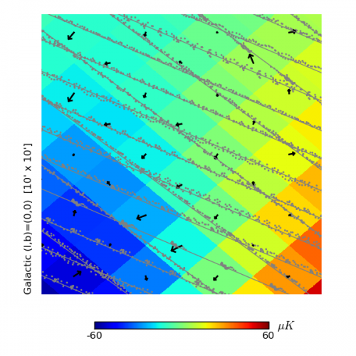
Planck-HFI maps are produced at HEALPix resolution 11 [math](N_{\rm side} = 2048)[/math], corresponding to pixels with a typical dimension of [math]1.7'[/math]. With the resolution comparable to the spacing between scanning rings there is an uneven distribution of hits within pixels, introducing a complication in the analysis and interpretation of the Planck maps. A sample of the Planck distribution of sample hits within pixels is illustrated in figure below.

Illustration of TOI samples near the Galactic plane (gray dots), over-plotted on a simulated CMB realization which has been convolved with a Gaussian 7' FWHM beam and pixelized at $(N_{\rm side} = 2048)$. Associated scanning rings (gray lines) as well as centers of mass for the hit distribution (black arrows) are also plotted.

The collaboration has produced 3 codes which may be used to simulate the effect of pixelization on the observed sky, LevelS/TotalConvoler/Conviqt, FeBeCoP, and FICSBell.

For the measurement of CMB fluctuations, the effects of pixelization may be studied analytically. On the small scales relevant to pixelization, the observed CMB is smooth, both due to physical damping as well as the convolution of the instrumental beam. Taylor expanding the CMB temperature about a pixel center to second order, the typical gradient amplitude is given by [math]\langle |\nabla T |^2 \rangle = \frac{1}{4\pi} \sum_{l} l(l+1)(2l+1) C_l^{T} W_l \approx 1\times10^9 \mu K^2 / {\rm rad}^2.[/math] where the approximate value is calculated for a [math]\Lambda[/math] CDM cosmology with a [math]7'[/math]FWHM Gaussian beam. The typical curvature of the observed temperature, on the other hand is given by [math]\langle |\nabla^2 T |^2 \rangle = \frac{1}{4\pi} \sum_{l} [l(l+1)]^2(2l+1) C_l^{T} W_l \approx 7\times10^{14} \mu K^2 / {\rm rad}^4.[/math] On the scales relevant to the maximum displacement from the center of a [math]1.7'[/math] pixel, the maximum displacement is [math]{\cal O}(1' = 3\times10^{-4} {\rm rad})[/math], and so the gradient term tends to dominate, although the curvature term is still non-negligible. For each observation of a pixel, we can denote the displacement from the pixel center as [math]d = d_{\theta} + i d_{\phi}[/math]. The average over all hits within a pixel gives an overall deflection vector which we will denote for a pixel center located at [math]\hat{n}[/math] as [math]d(\hat{n})[/math]. This represents the center of mass of the hit distribution; Fig. 2 shows these average deflections using black arrows. The deflection field [math]d(\hat{n})[/math] may be decomposed into spin-1 spherical harmonics as [math]d_{lm} = \int_{4\pi} {}_1 Y_{lm}^* d(\hat{n}).[/math] With a second order Taylor expansion of the CMB temperature about each pixel center, it is then possible to calculate the average pseudo-Cl power spectrum of the pixelized sky. This is given by

[math] C_l^{T} = [1-l(l+1)R^d] {C}_l^{T} W_l + \frac{1}{2} \sum_{l_1 l_2} \frac{l_1(l_1+1)(2l_1+1)(2l_2+1)}{4\pi} \left( \begin{array}{ccc} \! l_1\! & l_2\! & l\! \\ \! l\! & -l\! & 0\! \end{array} \right)^2 C_{l_1}^{T} W_{l_1} \left[ C_{l_2}^{d+} + (-1)^{l + l_1 + l_2} C_{l_2}^{ d-} \right], \label{eqn:clt_pixelized} [/math]

where [math]R^{d} = \langle |d|^2 \rangle/2[/math] is half the mean-squared deflection magnitude (averaged over hits within a pixel, as well as over pixels). [math]C_l^{d+}[/math] is the sum of the gradient and curl power spectra of [math]d_{lm}[/math], and [math]C_l^{d-}[/math] is the gradient spectrum minus the curl spectrum. The [math]R^{d}[/math] term describes a smearing of the observed sky due to pixelization. For uniform pixel coverage of [math]N_{\rm side}=2048[/math] pixels [math]\sqrt{ \langle |d|^2 \rangle } = 0.725'[/math] while, for the hit distribution of Planck frequency maps, [math]R^{d}[/math] is typically within 0.2% of this value for CMB channels, and 0.4% for all channels. This term is therefore accurately described by the HEALPix pixel window function, which is derived under the assumption of uniform pixel coverage, and the resulting relative error on the beam window function is at most [math]4\times 10^{-4}[/math] for [math]\ell \le 3000[/math].

The effect of pixelization is essentially degenerate with that of gravitational lensing of the CMB, with the difference that it (1) acts on the beam-convolved sky, rather than the actual sky and (2) produces a curl-mode deflection field as well as a gradient mode. This is discussed further in the Planck gravitational lensingPlanck-2013-XVII paper, where the subpixel deflection field constitutes a potential source of bias for the measured lensing potential. Indeed, Eq. \ref{eqn:clt_pixelized} is just a slightly modified version of the usual first order CMB lensing power spectrum Hu (2000), Lewis and Challinor (2006) to accommodate curl modes.

A useful approximation to Eq. \ref{eqn:clt_pixelized} which is derived in the unrealistic limit that the deflection vectors are uncorrelated between pixels, but in practice gives a good description of the power induced by the pixelization, is that the [math]d(\hat{n})[/math] couples the CMB gradient into a source of noise with an effective level given by [math]\sigma^{N} \approx \sqrt{ R^T \frac{4\pi}{N_{\rm pix}} \langle | d(\hat{n}) |^2 \rangle }, % (\muKarcmin ),[/math]

where the average is taken over all pixels and [math]R^T[/math] is half the mean-squared power in the CMB gradient: [math]R^{T} = \frac{1}{8\pi} \sum_{l} l(l+1)(2l+1) \tilde{C}_l^{T}.[/math] For frequency-combined maps, [math]\sqrt{ \langle | d(\hat{n}) |^2 \rangle }[/math] is typically on the order of [math]0.1'[/math], and so the induced noise is at the level of [math]\sigma^{N} \sim 2 \mu[/math]K arcmin. This is small compared to the instrumental contribution, although it does not disappear when taking cross-spectra, depending on how coherent the hit distributions of the two maps in the cross-spectrum are.