2015 CMB and astrophysical component maps
Contents
[hide]- 1 Overview
- 2 CMB maps
- 3 Astrophysical foregrounds from parametric component separation
- 4 CO emission maps
- 5 Modelling of the thermal dust emission with the Draine and Li dust model
- 6 Thermal dust and CIB all-sky maps from GNILC component separation
- 7 References
Overview[edit]
This section describes the maps of astrophysical components produced from the Planck data. These products are derived from some or all of the nine frequency channel maps described above using different techniques and, in some cases, using other constraints from external data sets. Here we give a brief description of each product and how it is obtained, followed by a description of the FITS file containing the data and associated information. All the details can be found in Planck-2015-A09[1] and Planck-2015-A10[2].
CMB maps[edit]
CMB maps have been produced using four different methods: COMMANDER, NILC, SEVEM, and SMICA, as described in the CMB and foreground separation section and also in Appendices A-D of Planck-2015-A09[1] and references therein.
As discussed extensively in Planck-2015-A01[3], Planck-2015-A06[4], Planck-2015-A08[5], and Planck-2015-A09[1], the residual systematics in the Planck 2015 polarization maps have been dramatically reduced compared to 2013, by as much as two orders of magnitude on large angular scales. Nevertheless, on angular scales greater than 10 degrees, correponding to l < 20, systematics are still non-negligible compared to the expected cosmological signal.
It was not possible, for this data release, to fully characterize the large-scale residuals from the data or from simulations. Therefore all results published by the Planck Collaboration in 2015 which are based on CMB polarization have used maps which have been high-pass filtered to remove the large angular scales. We warn all users of the CMB polarization maps that they cannot yet be used for cosmological studies at large angular scales.
For convenience, we provide as default polarized CMB maps from which all angular scales at l < 30 have been filtered out.
For each method we provide the following:
- Full-mission CMB intensity map, confidence mask and beam transfer function.
- Full-mission CMB polarisation map,
- A confidence mask.
- A beam transfer function.
In addition, and for characterisation purposes, we include six other sets of maps from three data splits: first/second half-ring, odd/even years and first/second half-mission. For the year-1,2 and half-mission-1,2 data splits we provide half-sum and half-difference maps which are produced by running the corresponding sums and differences inputs through the pipelines. The half-difference maps can be used to provide an approximate noise estimates for the full mission, but they should be used with caution. Each split has caveats in this regard: there are noise correlations between the half-ring maps, and missing pixels in the other splits. The Intensity maps are provided at Nside = 2048, at 5 arcmin resolution, while the Polarisation ones are provided at Nside = 1024, at 10 arcmin resolution. All maps are in units of Kcmb.
In addition, for each method we provide three sets of files, each categorized by the "R2.0X" label as follows:
- R2.02
This set of intensity and polarisation maps are provided at a resolution of Nside=1024. The Stokes Q and U maps are high-pass filtered to contain only modes above l > 30, as explained above and as used for analysis by the Planck Collaboration; THESE ARE THE POLARISATION MAPS WHICH SHOULD BE USED FOR COSMOLOGICAL ANALYSIS. Each type of map is packaged into a separate fits file (as for "R2.01"), resulting in file sizes which are easier to download (as opposed to the "R2.00" files), and more convenient to use with commonly used analysis software.
- R2.01
This is the most complete set of 2015 CMB maps, containing Intensity products at a resolution of Nside=2048, and both Intensity and Polarisation at resolution of Nside=1024. For polarisation (Q and U), they contain all angular resolution modes. WE CAUTION USERS ONCE AGAIN THAT THE STOKES Q AND U MAPS ARE NOT CONSIDERED USEABLE FOR COSMOLOGICAL ANALYSIS AT l < 30. The structure of these files is the same as for "R2.02".
- R2.00
This set of files is equivalent to the "R2.01" set, but are packaged into only two large files. Warning: downloading these files could be very lengthy...
For a complete description of the above data structures, see below; the content of the first extensions is illustrated and commented in the table below.
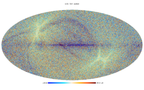
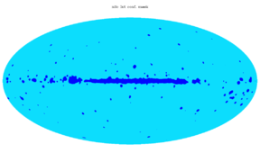
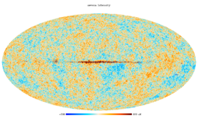
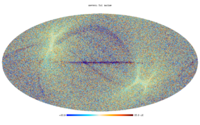
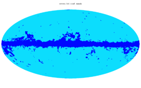
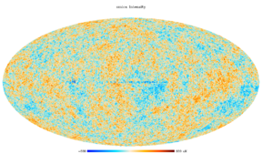
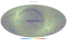
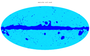
The gallery below shows the Intensity, noise from half-mission, half-difference, and confidence mask for the four pipelines, in the order COMMANDER, NILC, SEVEM and SMICA, from top to bottom. The Intensity maps' scale is [–500.+500] μK, and the noise spans [–25,+25] μK. We do not show the Q and U maps since they have no significant visible structure to contemplate.
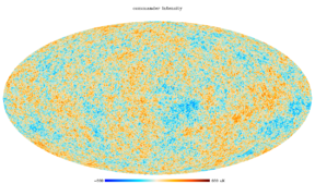
commander temperature
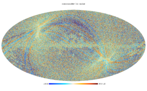
commander noise
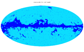
commander mask
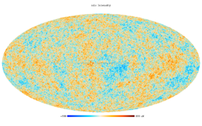
nilc temperature
nilc noise
nilc mask
sevem temperature
sevem noise
sevem mask
smica temperature
smica noise
smica mask


Product description[edit]
COMMANDER[edit]
- Principle
- COMMANDER is a Planck software code implementing pixel based Bayesian parametric component separation. Each astrophysical signal component is modelled in terms of a small number of free parameters per pixel, typically in terms of an amplitude at a given reference frequency and a small set of spectral parameters, and these are fitted to the data with an MCMC Gibbs sampling algorithm. Instrumental parameters, including calibration, bandpass corrections, monopole and dipoles, are fitted jointly with the astrophysical components. A new feature in the Planck 2015 analysis is that the astrophysical model is derived from a combination of Planck, WMAP and a 408 MHz (Haslam et al. 1982) survey, providing sufficient frequency support to resolve the low-frequency components into synchrotron, free-free and spinning dust. For full details, see Planck-2015-A10[2].
- Resolution (effective beam)
- The Commander sky maps have different angular resolutions depending on data products:
- The components of the full astrophysical sky model derived from the complete data combination (Planck, WMAP, 408 MHz) have a 1 degree FWHM resolution, and are pixelized at Nside=256. The corresponding CMB map defines the input map for the low-l Planck 2015 temperature likelihood.
- The Commander CMB temperature map derived from Planck-only observations has an angular resolution of ~5 arcmin and is pixelized at Nside=2048. This map is produced by harmonic space hybridiziation, in which independent solutions derived at 40 arcmin (using 30-857 GHz data), 7.5 arcmin (using 143-857 GHz data), and 5 arcmin (using 217-857 GHz data) are coadded into a single map.
- The Commander CMB polarization map has an angular resolution of 10 arcmin and is pixelized at Nside=1024. As for the temperature case, this map is produced by harmonic space hybridiziation, in which independent solutions derived at 40 arcmin (using 30-353 GHz data) and 10 arcmin (using 100-353 GHz data) are coadded into a single map.
- Confidence mask
- The Commander confidence masks are produced by thresholding the chi-square map characterizing the global fits, combined with direct CO amplitude thresholding to eliminate known leakage effects. In addition, we exclude the 9-year WMAP point source mask in the temperature mask. For full details, see Sections 5 and 6 in Planck-2015-A10[2]. A total of 81% of the sky is admitted for high-resolution temperature analysis, and 83% for polarization analysis. For low-resolution temperature analysis, for which the additional WMAP and 408 MHz observations improve foreground constraints, a total of 93% of the sky is admitted.
NILC[edit]
- Principle
- The Needlet-ILC (hereafter NILC) CMB map is constructed both in total intensity as well as polarization: Q and U Stokes parameters. For total intensity, all Planck frequency channels are included. For polarization, all polarization sensitive frequency channels are included, from 30 to 353 GHz. The solution, for T, Q and U is obtained by applying the Internal Linear Combination (ILC) technique in needlet space, that is, with combination weights which are allowed to vary over the sky and over the whole multipole range.
- Resolution (effective beam)
- The spectral analysis, and estimation of the NILC coefficients, is performed up to a maximum . The effective beam is equivalent to a Gaussian circular beam with FWHM=5 arcminutes.
- Confidence mask
- The same procedure is followed by SMICA and NILC for producing confidence masks, though with different parametrizations. A low resolution smoothed version of the NILC map, noise subtracted, is thresholded to 73.5 squared micro-K for T, and 6.75 squared micro-K for Q and U.
SEVEM[edit]
- Principle
- SEVEM produces clean CMB maps at several frequencies by using a procedure based on template fitting in real space. The templates are typically constructed from the lowest and highest Planck frequencies and then subtracted from the CMB-dominated channels, with coefficients that are chosen to minimize the variance of the clean map outside a considered mask. In the cleaning process, no assumptions about the foregrounds or noise levels are needed, rendering the technique very robust. Two single frequency clean maps are then combined to obtain the final CMB map.
- Resolution
- For intensity the clean CMB map is constructed up to a maximum at Nside=2048 and at the standard resolution of 5 arcminutes (Gaussian beam).
- For polarization the clean CMB map is produced at Nside=1024 with a resolution of 10 arcminutes (Gaussian beam) and a maximum .
- Confidence masks
- The confidence masks cover the most contaminated regions of the sky, leaving approximately 85 per cent of useful sky for intensity, and 80 per cent for polarization.
Foregrounds-subtracted maps[edit]
In addition to the regular CMB maps, SEVEM provides maps cleaned of the foregrounds for selected frequency channels (categorized as fgsub-sevem in the archive). In particular, for intensity there are clean CMB maps available at 100, 143 and 217 GHz, provided at the original resolution of the uncleaned channel and at Nside=2048. For polarization, there are Q/U clean CMB maps for the 70, 100 and 143 GHz (at Nside=1024). The 70 GHz clean map is provided at its original resolution, whereas the 100 and 143 GHz maps have a resolution given by a Gaussian beam with fwhm=10 arcminutes.
SMICA[edit]
- Principle
- SMICA produces CMB maps by linearly combining all Planck input channels with multipole-dependent weights. It includes multipoles up to . Temperature and polarization maps are produced independently.
- Resolution (effective beam)
- The SMICA intensity map has an effective beam window function of 5 arc-minutes which is truncated at and is not deconvolved from the pixel window function. Thus the delivered beam window function is the product of a Gaussian beam at 5 arcminutes and the pixel window function for =2048.
- The SMICA Q and U maps are obtained similarly but are produced at =1024 with an effective beam of 10 arc-minutes (to be multiplied by the pixel window function, as for the intensity map).
- Confidence mask
- A confidence mask is provided which excludes some parts of the Galactic plane, some very bright areas and masked point sources. This mask provides a qualitative (and subjective) indication of the cleanliness of a pixel. See section below detailing the production process.
Common Masks[edit]
A number of common masks have been defined for analysis of the CMB temperature and polarization maps. They are based on the confidence masks provided by the component separation methods. One mask for temperature and one mask for polarization have been chosen as the preferred masks based on subsequent analyses.
The common masks for the CMB temperature maps are:
- UT78: union of the Commander, SEVEM, and SMICA temperature confidence masks (the NILC mask was not included since it masks much less of the sky). It has fsky = 77.6%. This is the preferred mask for temperature.
- UTA76: in addition to the UT78 mask, it masks pixels where standard deviation between the four CMB maps is greater than 10 μK. It has fsky = 76.1%.
The common masks for the CMB polarization maps are:
- UP78: the union of the Commander, SEVEM and SMICA polarization confidence masks (the NILC mask was not included since it masks much less of the sky). It has fsky = 77.6%.
- UPA77: In addition to the UP78 mask, it masks pixels where the standard deviation between the four CMB maps, averaged in Q and U, is greater than 4 μK. It has fsky = 76.7%.
- UPB77: in addition to the UP78 mask, it masks polarized point sources detected in the frequency channel maps. It has fsky = 77.4%. This is the preferred mask for polarization.
CMB-subtracted frequency maps ("Foreground maps")[edit]
These are the full-sky, full-mission frequency maps in intensity from which the CMB has been subtracted. The maps contain foregrounds and noise. They are provided for each frequency channel and for each component separation method. They are grouped into 8 files, two for each method of which there is one for each instrument. The maps are are at Nside = 1024 for the three LFI channels and at Nside = 2048 for the six HFI channels. The filenames are:
- LFI_Foregrounds-{method}_1024_Rn.nn.fits (145 MB each)
- HFI_Foregrounds-{method}_2048_Rn.nn.fits (1.2 GB each)
To remove the CMB, the respective CMB map was first deconvolved with the 5 arcmin beam, then convolved with the beam of the frequency channel, and finally subtracted from the frequency map. This was done using the in harmonic space, assuming a symmetric beam.
The CMB-subtracted maps have complicated noise properties. The CMB maps contain a noise contribution from each of the frequency maps, depending on the weights with which they were combined. Therefore subtracting the CMB map from a frequency channel contributes additional noise from the other frequency channels.
The frequency maps from which the CMB have been subtracted are:
- LFI_SkyMap_0nn_1024_R2.01_full.fits
- HFI_SkyMap_nnn_2048_R2.0n_full.fits
Note that the temperature column in the HFI R2.00, R2.01 and R2.02 is the same, since the changes in these maps involved the polarization columns only. Also note that the zodiacal light correction described here was applied to the HFI temperature maps before the CMB subtraction.
Quadrupole Residual Maps[edit]
The second-order (kinematic) quadrupole is a frequency-dependent effect. During the production of the frequency maps the frequency-independent part was subtracted, which leaves a frequency-dependent residual quadrupole. The residuals in the component-separated CMB temperature maps have been estimated by simulating the effect in the frequency maps and propagating it through the component separation pipelines. The residuals have an amplitude of around 2 μK peak-to-peak. The maps of the estimated residuals can be used to remove the effect by subtracting them from the CMB maps.
Production process[edit]
COMMANDER[edit]
- Pre-processing
- All sky maps are first convolved to a common resolution that is larger than the largest beam of any frequency channel. For the combined Planck, WMAP and 408 MHz temperature analysis, the common resolution is 1 degree FWHM; for the Planck-only, all-frequency analysis it is 40 arcmin FWHM; and for the intermediate-resolution analysis it is 7.5 arcmin; while for the full-resolution analysis, we assume all frequencies between 217 and 857 GHz have a common resolution, and no additional convolution is performed. For polarization, only two smoothing scales are employed, 40 and 10 arcmin, respectively. The instrumental noise rms maps are convolved correspondingly, properly accouting for their matrix-like nature.
- Priors
- The following priors are enforced in the Commander analysis:
- All foreground amplitudes are enforced to be positive definite in the low-resolution analysis, while no amplitude priors are enforced in the high-resolution analyses
- Monopoles and dipoles are fixed to nominal values for a small set of reference frequencies
- Gaussian priors are enforced on spectral parameters, with values informed by the values derived in the high signal-to-noise areas of the sky
- The Jeffreys ignorance prior is enforced on spectral parameters in addition to the informative Gaussian priors
- Fitting procedure
- Given data and priors, Commander either maximizes, or samples from, the Bayesian posterior, P(theta|data). Because this is a highly non-Gaussian and correlated distribution, involving millions of parameters, these operations are performed by means of the Gibbs sampling algorithm, in which joint samples from the full distributions are generated by iteratively sampling from the corresponding conditional posterior distributions, P(theta_i| data, theta_{j/=i}). For the low-resolution analysis, all parameters are optimized jointly, while in the high-resolution analyses, which employs fewer frequency channels, low signal-to-noise parameters are fixed to those derived at low resolution. Examples of such parameters include monopoles and dipoles, calibration and bandpass parameters, thermal dust temperature etc.
NILC[edit]
- Pre-processing
- All sky frequency maps are deconvolved using the DPC beam transfer function provided, and re-convolved with a 5 arcminutes FWHM circular Gaussian beam. In polarization, prior to the smoothing process, all sky E and B maps are derived from Q and U using standard HEALPix tools from each individual frequency channels
- Linear combination
- Pre-processed input frequency maps are decomposed in needlet coefficients, specified in the Appendix B of the Planck A11 paper, with shape given by Table B.1. Minimum variance coefficients are then obtained, using all channels for T, from 30 to 353 for E and B.
- Post-processing
- E and B maps are re-combined into Q and U products using standard HEALPix tools.
SEVEM[edit]
The templates used in the SEVEM pipeline are typically constructed by subtracting two close Planck frequency channel maps, after first smoothing them to a common resolution to ensure that the CMB signal is properly removed. A linear combination of the templates is then subtracted from (hitherto unused) map d to produce a clean CMB map at that frequency. This is done in real space at each position on the sky: where is the number of templates. The coefficients are obtained by minimising the variance of the clean map outside a given mask. Note that the same expression applies for I, Q and U. Although we exclude very contaminated regions during the minimization, the subtraction is performed for all pixels and, therefore, the cleaned maps cover the full-sky (although we expect that foreground residuals are present in the excluded areas).
There are several possible configurations of SEVEM with regard to the number of frequency maps which are cleaned or the number of templates that are used in the fitting. Note that the production of clean maps at different frequencies is of great interest in order to test the robustness of the results, and these intermediate products (clean maps at individual frequencies for intensity and polarization) are also provided in the archive. Therefore, to define the best strategy, one needs to find a compromise between the number of maps that can be cleaned independently and the number of templates that can be constructed.
- Intensity
For the CMB intensity map, we have cleaned the 100 GHz, 143 GHz and 217 GHz maps using a total of four templates. Three of them are constructed as the difference of two consecutive Planck channels smoothed to a common resolution (30-44, 44-70 and 545-353) while the 857 GHz channel is chosen as the fourth template. First of all, the six frequency channels which are going to be part of the templates are inpainted at the point source positions detected using the Mexican Hat Wavelet algorithm. The size of the holes to be inpainted is determined taking into account the beam size of the channel as well as the flux of each source. The inpainting algorithm is based on simple diffuse inpainting, which fills one pixel with the mean value of the neighbouring pixels in an iterative way. To avoid inconsistencies when subtracting two channels, each frequency map is inpainted on the sources detected in that map and on the second map (if any) used to construct the template. Then the maps are smoothed to a common resolution (the first channel in the subtraction is smoothed with the beam of the second map and viceversa). For the 857 GHz template, we simply filter the inpainted map with the 545 GHz beam.
The coefficients are obtained by minimising the variance outside the analysis mask, that covers the 1 per cent brightest emission of the sky as well as point sources detected at all frequency channels. Once the maps are cleaned, each of them is inpainted on the point sources positions detected at that (raw) channel. Then, the MHW algorithm is run again, now on the clean maps. A relatively small number of new sources are found and are also inpainted at each channel. The resolution of the clean map is the same as that of the original data. Our final CMB map is then constructed by combining the 143 and 217 GHz maps by weighting the maps in harmonic space taking into account the noise level, the resolution and a rough estimation of the foreground residuals of each map (obtained from realistic simulations). This final map has a resolution corresponding to a Gaussian beam of fwhm=5 arcminutes.
In addition, the clean CMB maps produced at 100, 143 and 217 GHz frequencies are also provided. The resolution of these maps is the same as that of the uncleaned frequency channels and have been constructed at Nside=2048. They have been inpainted at the position of the detected point sources. Note that these three clean maps should be close to independent, although some level of correlation will be present since the same templates have been used to clean the maps.
The confidence mask is produced by studying the differences between several SEVEM CMB reconstructions, which correspond to maps cleaned at different frequencies or using different analysis masks. The obtained mask leaves a useful sky fraction of approximately 85 per cent.
- Polarization
To clean the polarization maps, a procedure similar to the one used for intensity data is applied to the Q and U maps independently. However, given that a narrower frequency coverage is available for polarization, the selected templates and maps to be cleaned are different. In particular, we clean the 70, 100 and 143 GHz using three templates for each channel. The first step of the pipeline is to inpaint the positions of the point sources using the MHW, in those channels which are going to be used in the construction of templates, following the same procedure as for the intensity case. The inpainting is performed in the frequency maps at their native resolution. These inpainted maps are then used to construct a total of four templates. To trace the synchrotron emission, we construct a template as the subtraction of the 30 GHz minus the 44 GHz map, after being convolved with the beam of each other. For the dust emission, the following templates are considered: 353-217 GHz (smoothed at 10' resolution), 217-143 GHz (used to clean 70 and 100 GHz) and 217-100 GHz (to clean 143 GHz). These two last templates are constructed at 1 degree resolution since an additional smoothing becomes necessary in order to increase the signal-to-noise ratio of the template. Conversely to the intensity case and due to the lower availability of frequency channels, it becomes necessary to use the maps to be cleaned as part of one of the templates. In this way, the 100 GHz map is used to clean the 143 GHz frequency channel and viceversa, making the clean maps less independent between them than in the intensity case.
These templates are then used to clean the non-inpainted 70 (at its native resolution), 100 (at 10' resolution) and 143 GHz maps (also at 10'). The corresponding linear coefficients are estimated independently for Q and U by minimising the variance of the clean maps outside a mask, that covers point sources and the 3 per cent brightest Galactic emission. Once the maps have been cleaned, inpainting of the point sources detected at the corresponding raw maps is carried out. The size of the holes to be inpainted takes into account the additional smoothing of the 100 and 143 GHz maps. The 100 and 143 GHz clean maps are then combined in harmonic space, using E and B decomposition, to produce the final CMB maps for the Q and U components at a resolution of 10' (Gaussian beam) for a HEALPix parameter Nside=1024. Each map is weighted taking into account its corresponding noise level at each multipole. Finally, before applying the post-processing HPF to the clean polarization data, the region with the brightest Galactic residuals is inpainted (5 per cent of the sky) to avoid the introduction of ringing around the Galactic centre in the filtering process.
The clean CMB maps at individual frequency channels produced as intermediate steps of SEVEM are also provided for Q and U, constructed at Nside=1024. The clean 70 GHz map is provided at its native resolution, while the clean maps at 100 and 143 GHz frequencies have a resolution of 10 arcminutes (Gaussian beam). The three maps have been inpainted in the positions of the detected point sources. Note that, due to the availability of a smaller number of templates for polarization than for intensity, these maps are less independent than for the temperature case, since, for instance, the 100 GHz map is used to clean the 143 GHz one and viceversa.
The confidence mask includes all the pixels above a given threshold in a smoothed version of the clean CMB map, the regions more contaminated by the CO emission and those pixels more affected by the high-pass filtering, leaving a useful sky fraction of approximately 80 per cent.
SMICA[edit]
A) Production of the intensity map.
- 1) Pre-processing
- Before computing spherical harmonic coefficients, all input maps undergo a pre-processing step to deal with regions of very strong emission (such as the Galactic center) and point sources. The point sources with SNR > 5 in the PCCS catalogue are fitted in each input map. If the fit is successful, the fitted point source is removed from the map; otherwise it is masked and the hole is filled in by a simple diffusive process to ensure a smooth transition and mitigate spectral leakage. The diffusive inpainting process is also applied to some regions of very strong emissions. This is done at all frequencies but 545 and 857 GHz, here all point sources with SNR > 7.5 are masked and filled-in similarly.
- 2) Linear combination
- The nine pre-processed Planck frequency channels from 30 to 857 GHz are harmonically transformed up to and co-added with multipole-dependent weights as shown in the figure.
- 3) Post-processing
- A confidence mask is determined (see the Planck paper) and all regions which have been masked in the pre-processing step are added to it.
B) Production of the Q and U polarisation maps.
The SMICA pipeline for polarization uses all the 7 polarized Planck channels. The production of the Q and U maps is similar to the production of the intensity map. However, there is no input point source pre-processing of the input maps. The regions of very strong emission are masked out using an apodized mask before computing the E and B modes of the input maps and combining them to produce the E and B modes of the CMB map. Those modes are then used to synthesize the U and Q CMB maps. The E and B parts of the input frequency maps being processed jointly, there are, at each multipole, 2*7=14 coefficients (weights) defined to produce the E modes of the CMB map and as many to produce the B part. The weights are displayed in the figure below. The Q and U maps were originally produced at Nside=2048 with a 5-arc-minute resolution, but were downgraded to Nside=1024 with a 10 arc-minute resolution for this release.
Masks[edit]
Summary table with the different masks that have been used by the component separation methods to pre-process and to process the frequency maps and the CMB maps.
| Commander 2015 (PR2) | Used for diffuse inpainting of input frequency maps | Used for constrained Gaussian realization inpaiting of CMB map | Description |
|---|---|---|---|
| TMASK | NO | NO | TMASK (the equivalent to PR1 VALMASK) is the confidence mask in temperature that defines the region where the reconstructed CMB is trusted. It can be found inside COM_CMB_IQU-commander-field-Int_2048_R2.01_full.fits. |
| PMASK | NO | NO | PMASK is the confidence mask in polarization that defines the region where the reconstructed CMB is trusted. It can be found inside COM_CMB_IQU-commander_1024_R2.02_full.fits. |
| INP_MASK_T | NO | YES | Three masks have been used for inpaiting of CMB maps for specific ranges: three different angular resolution maps (40 arcmin, 7.5 arcmin and full resolution), are produced using different data combinations and foreground models. Each of these are inpainted with their own masks with a constrained Gaussian realization before coadding the three maps in harmonic space. |
| INP_MASK_P | NO | YES | Mask used for inpainting of the CMB map in polarization. |
| SEVEM 2015 (PR2) | Used for Diffuse Inpainting of foregorund subtracted CMB maps (fgsub-sevem) | Used for constrained Gaussian realization inpaiting of CMB map | Description |
| TMASK | NO | NO | TMASK (the equivalent to PR1 VALMASK) is the confidence mask in temperature that defines the region where the reconstructed CMB is trusted. It can be found inside COM_CMB_IQU-sevem-field-Int_2048_R2.01_full.fits. |
| PMASK | NO | NO | PMASK is the confidence mask in polarization that defines the region where the reconstructed CMB is trusted. It can be found inside COM_CMB_IQU-sevem_1024_R2.02_full.fits. |
| INP_MASK_T | YES | NO | Point source mask for temperature. This mask is the combination of the 143 and 217 T point source masks used for the inpainting of the foreground subtracted CMB maps at those two frequencies. These two maps have been combined to produce the final CMB map. |
| INP_MASK_P | YES | NO | Point source mask for polarization. This mask is the combination of the 100 and 143 point source masks used for the inpainting of the foreground subtracted CMB maps at those two frequencies. These two maps have been combined to produce the final CMB map. |
| INP_MASK_T for the cleaned 100, 143 and 217 GHz CMB | YES | NO | Three temperature point source masks used for the inpainting of the foreground subtracted CMB maps at the considered frequencies:
|
| INP_MASK_P for the cleaned 70, 100 and 143 GHz CMB | YES | NO | Three polarization point source masks used for the inpainting of the foreground subtracted CMB maps at the considered frequencies: |
| NILC 2015 (PR2) | Used for diffuse inpainting of input frequency maps | Used for constrained Gaussian realization inpaiting of CMB map | Description |
| TMASK | NO | NO | TMASK (the equivalent to PR1 VALMASK) is the confidence mask in temperature that defines the region where the reconstructed CMB is trusted. It can be found inside COM_CMB_IQU-nilc-field-Int_2048_R2.01_full.fits. |
| PMASK | NO | NO | PMASK is the confidence mask in polarization that defines the region where the reconstructed CMB is trusted. It can be found inside COM_CMB_IQU-nilc_1024_R2.02_full.fits. |
| INP_MASK | YES | NO | The pre-processing involves inpainting of the holes in INP_MASK in the frequency maps prior to applying NILC on them. The first mask (nside 2048) has been used for the pre-processing of sky maps for HFI channels and second one for LFI channels (nside 1024). They can downloaded here:
COM_Mask_PointSrcGalplane_nilc_dx11_preproc_1024_R2.00.fits COM_Mask_PointSrcGalplane_nilc_dx11_preproc_2048_R2.00.fits |
| SMICA 2015 (PR2) | Used for diffuse inpainting of input frequency maps | Used for constrained Gaussian realization inpaiting of CMB map | Description |
| TMASK | NO | YES | TMASK (the equivalent to PR1 VALMASK) is the confidence mask in temperature that defines the region where the reconstructed CMB is trusted. It can be found inside COM_CMB_IQU-smica-field-Int_2048_R2.01_full.fits. |
| PMASK | NO | YES | PMASK is the confidence mask in polarization that defines the region where the reconstructed CMB is trusted. It can be found inside COM_CMB_IQU-smica_1024_R2.02_full.fits. |
| I_MASK | YES | NO | I_MASK, as in PR1, defines the regions over which CMB is not built. It is a combination of point source masks, Galactic plane mask and other bright regions like LMC, SMC, etc. It can downloaded here: COM_Mask_PointSrcGalplane_smica_harmonic_mask_2048_R2.00.fits |
Inputs[edit]
The input maps are the sky temperature maps described in the Sky temperature maps section. SMICA and SEVEM use all the maps between 30 and 857 GHz; NILC uses the ones between 44 and 857 GHz. Commander-Ruler uses frequency channel maps from 30 to 353 GHz.
File names and structure[edit]
Three sets of files FITS files containing the CMB products are available. In the first set all maps (i.e., covering different parts of the mission) and all characterisation products for a given method and a given Stokes parameter are grouped into a single extension, and there are two files per method (smica, nilc, sevem, and commander), one for the high resolution data (I only, Nside=2048) and one for low resolution data (Q and U only, Nside=1024). Each file also contains the associated confidence mask(s) and beam transfer function. These are the R2.00 files which have names like
- COM_CMB_IQU-{method}-field-{Int,Pol}_Nside_R2.00.fits
There are 7 coverage periods:full, halfyear-1,2, halfmission-1,2, or ringhalf-1,2, and 4 characterisation products: half-sum and half-difference for the year and the half-mission periods.
In the second second set the different coverages are split into different files which in most cases have a single extension with I only (Nside=1024) and I, Q, and U (Nside=1024). This second set was built in order to allow users to use standard codes like spice or anafast on them, directly. So this set contains the I maps at Nside=1024, which are not contained in the R2.00; on the other hand this set does not contain the half-sum and half-difference maps. These are the 2.01 files which have names like
- COM_CMB_IQU-{method}{-field-Int|Pol}_Nside_R2.01_{coverage}.fits for the regular CMB maps, and
- COM_CMB_IQU-{fff}-{fgsub-sevem}{-field-Int|Pol}_Nside_R2.01_{coverage}.fits for the sevem frequency-dependent, foregrounds-subtracted maps,
where field-Int|Pol is used to indicate that only Int or only Pol data are contained (at present only field-Int is used for the high-res data), and is not included in the low-res data which contains all three Stokes parameters, and coverage is one of full, halfyear-1,2, halfmission-1,2, or ringhalf-1,2. Also, the coverage=full files contain also the confidence mask(s) and beam transfer function(s) which are valid for all products of the same method (one for Int and one for Pol when both are available).
The third set has the same structure as the Nside=1024 products of R2.01, but the Q and U maps have been high-pass filtered to remove modes at l < 30 for the reasons indicated earlier. These are the default products for use in polarisation studies. They are the R2.02 files which have names like:
- COM_CMB_IQU-{method}_1024_R2.02_{coverage}.fits
Version 2.00 files[edit]
These have names like
- COM_CMB_IQU-{method}-field-{Int,Pol}_Nside_R2.00.fits,
as indicated above. They contain:
- a minimal primary extension with no data;
- one or two BINTABLE data extensions with a table of Npix lines by 14 columns in which the first 13 columns is a CMB maps produced from the full or a subset of the data, as described in the table below, and the last column in a confidence mask. There is a single extension for Int files, and two, for Q and U, for Pol files.
- a BINTABLE extension containing the beam transfer function (mistakenly called window function in the files).
If Nside=1024 the files contain I, Q and U maps, whereas if Nside=2048 only the I map is given.
| Ext. 1. or 2. EXTNAME = COMP-MAP (BINTABLE) | |||
|---|---|---|---|
| Column Name | Data Type | Units | Description |
| I or Q or U | Real*4 | uK_cmb | I or Q or U map |
| HM1 | Real*4 | uK_cmb | Half-miss 1 |
| HM2 | Real*4 | uK_cmb | Half-miss 2 |
| YR1 | Real*4 | uK_cmb | Year 1 |
| YR2 | Real*4 | uK_cmb | Year 2 |
| HR1 | Real*4 | uK_cmb | Half-ring 1 |
| HR2 | Real*4 | uK_cmb | Half-ring 2 |
| HMHS | Real*4 | uK_cmb | Half-miss, half sum |
| HMHD | Real*4 | uK_cmb | Half-miss, half diff |
| YRHS | Real*4 | uK_cmb | Year, half sum |
| YRHD | Real*4 | uK_cmb | Year, half diff |
| HRHS | Real*4 | uK_cmb | Half-ring half sum |
| HRHD | Real*4 | uK_cmb | Half-ring half diff |
| MASK | BYTE | Confidence mask | |
| Keyword | Data Type | Value | Description |
| AST-COMP | String | CMB | Astrophysical compoment name |
| PIXTYPE | String | HEALPIX | |
| COORDSYS | String | GALACTIC | Coordinate system |
| POLCCONV | String | COSMO | Polarization convention |
| ORDERING | String | NESTED | Healpix ordering |
| NSIDE | Int | 1024 or 2048 | Healpix Nside |
| METHOD | String | name | Cleaning method (smica/nilc/sevem/commander) |
| Ext. 2. or 3. EXTNAME = BEAM_WF (BINTABLE) . See Note 1 | |||
| Column Name | Data Type | Units | Description |
| BEAMWF | Real*4 | none | The effective beam transfer function, including the pixel window function. See Note 2. |
| Keyword | Data Type | Value | Description |
| LMIN | Int | value | First multipole of beam TF |
| LMAX | Int | value | Last multipole of beam TF |
| METHOD | String | name | Cleaning method (SMICA/NILC/SEVEM/COMMANDER-Ruler) |
Notes:
- Actually this is a beam transfer function, so BEAM_TF would have been more appropriate.
- The beam transfer function given here includes the pixel window function for the Nside=2048 pixelization. It means that, ideally, . The beam Window function is given by
Version 2.01 files[edit]
These files have names like:
- COM_CMB_IQU-{method}{-field-Int|Pol}_Nside_R2.01_{coverage}.fits for the regular CMB maps, and
- COM_CMB_IQU-{fff}-{fgsub-sevem}{-field-Int|Pol}_Nside_R2.01_{coverage}.fits for the sevem frequency-dependent, foregrounds-subtracted maps,
as indicated above. They contain:
- a minimal primary extension with no data, but with a NUMEXT keyword giving the number of extensions contained.
- one or two BINTABLE data extensions with a table of Npix lines by 1-5 columns depending on the file, as described above: the minimum begin I only, the maximum begin I, Q, U, and confidence masks for I and P.
- a BINTABLE extension containing the beam transfer function(s): one for I, and a second one that applies to both Q and U, if Nslde=1024.
If Nside=1024 the files contain I, Q and U maps, whereas if Nside=2048 only the I map is given. The basic structure, including information on the most important keywords, is given in the table below. For full details, see the FITS header.
| Ext. 1. or 2. EXTNAME = COMP-MAP (BINTABLE) | |||
|---|---|---|---|
| Column Name | Data Type | Units | Description |
| I_Stokes | Real*4 | uK_cmb | I map (Nside=1024,2048) |
| Q_Stokes | Real*4 | uK_cmb | Q map (Nside=1024) |
| U_Stokes | Real*4 | uK_cmb | U map (Nside=2048) |
| TMASK | Int | none | optional Temperature confidence mask |
| PMASK | Int | none | optional Polarisation confidence mask |
| Keyword | Data Type | Value | Description |
| AST-COMP | String | CMB | Astrophysical compoment name |
| PIXTYPE | String | HEALPIX | |
| COORDSYS | String | GALACTIC | Coordinate system |
| POLCCONV | String | COSMO | Polarization convention |
| ORDERING | String | NESTED | Healpix ordering |
| NSIDE | Int | 1024 or 2048 | Healpix Nside |
| METHOD | String | name | Cleaning method (SMICA/NILC/SEVEM) |
| Optional Ext. 2. or 3. EXTNAME = BEAM_TF (BINTABLE) | |||
| Column Name | Data Type | Units | Description |
| INT_BEAM | Real*4 | none | Effective beam transfer function. See Note 1. |
| POL_BEAM | Real*4 | none | Effective beam transfer function. See Note 1. |
| Keyword | Data Type | Value | Description |
| LMIN | Int | value | First multipole of beam WF |
| LMAX_I | Int | value | Last multipole for Int beam TF |
| LMAX_P | Int | value | Last multipole for Pol beam TF |
| METHOD | String | name | Cleaning method |
Notes:
- The beam transfer function given here includes the pixel window function for the Nside=2048 pixelization. It means that, ideally, . The beam Window function is given by
Version 2.02 files[edit]
For polarisation work, this is the default set of files to be used for cosmological analysis. Their content is identical to the "R2.01" files, except that angular scales above l < 30 have been filtered out of the Q and U maps.
These files have names like:
- COM_CMB_IQU-{method}_1024_R2.02_{coverage}.fits
as indicated above. They contain: The files contain
- a minimal primary extension with no data, but with a NUMEXT keyword giving the number of extensions contained.
- one or two BINTABLE data extensions with a table of Npix lines by 1-5 columns depending on the file, as described above: the minimum begin I only, the maximum begin I, Q, U, and confidence masks for I and P.
- a BINTABLE extension containing 2 beam transfer functions: one for I and one that applies to both Q and U.
If Nside=1024 the files contain I, Q and U maps, whereas if Nside=2048 only the I map is given. The basic structure, including information on the most important keywords, is given in the table below. For full details, see the FITS header.
| Ext. 1. or 2. EXTNAME = COMP-MAP (BINTABLE) | |||
|---|---|---|---|
| Column Name | Data Type | Units | Description |
| I_Stokes | Real*4 | uK_cmb | I map (Nside=1024) |
| Q_Stokes | Real*4 | uK_cmb | Q map (Nside=1024) |
| U_Stokes | Real*4 | uK_cmb | U map (Nside=2048) |
| TMASK | Int | none | optional Temperature confidence mask |
| PMASK | Int | none | optional Polarisation confidence mask |
| Keyword | Data Type | Value | Description |
| AST-COMP | String | CMB | Astrophysical compoment name |
| PIXTYPE | String | HEALPIX | |
| COORDSYS | String | GALACTIC | Coordinate system |
| POLCCONV | String | COSMO | Polarization convention |
| ORDERING | String | NESTED | Healpix ordering |
| NSIDE | Int | 1024 or 2048 | Healpix Nside |
| METHOD | String | name | Cleaning method (SMICA/NILC/SEVEM) |
| Optional Ext. 2. or 3. EXTNAME = BEAM_TF (BINTABLE) | |||
| Column Name | Data Type | Units | Description |
| INT_BEAM | Real*4 | none | Effective beam transfer function. See Note 1. |
| POL_BEAM | Real*4 | none | Effective beam transfer function. See Note 1. |
| Keyword | Data Type | Value | Description |
| LMIN | Int | value | First multipole of beam WF |
| LMAX_I | Int | value | Last multipole for Int beam TF |
| LMAX_P | Int | value | Last multipole for Pol beam TF |
| METHOD | String | name | Cleaning method |
Notes:
- The beam transfer function given here includes the pixel window function for the Nside=2048 pixelization. It means that, ideally, . The beam Window function is given by
The Common Masks[edit]
The common masks are stored into two different files for Temperature and Polarisation respectively:
- COM_CMB_IQU-common-field-MaskInt_2048_R2.nn.fits with the UT78 and UTA76 masks
- COM_CMB_IQU-common-field-MaskPol_1024_R2.nn.fits with the UP78, UPA77, and UPB77 masks
Both files contain also a map of the missing pixels for the half mission and year coverage periods. The 2 (for Temp) or 3 (for Pol) masks and the missing pixels maps are stored in 4 or 5 column a BINTABLE extension 1 of each file, named MASK-INT and MASK-POL, respectively. See the FITS file headers for details.
Quadrupole residual maps[edit]
The quadrupole residual maps are stored in files called:
- COM_CMB_IQU-kq-resid-{method}-field-Int_2048_R2.02.fits
They contain:
- a minimal primary extension with no data, but with a NUMEXT keyword giving the number of extensions contained.
- a single BINTABLE extension with a single column of Npix lines containing the HEALPIX map indicated
The basic structure of the data extension is shown below. For full details see the extension header.
| Ext. 1. EXTNAME = COMP-MAP (BINTABLE) | |||
|---|---|---|---|
| Column Name | Data Type | Units | Description |
| INTENSITY | Real*4 | K_cmb | the residual map |
| Keyword | Data Type | Value | Description |
| AST-COMP | String | KQ-RESID | Astrophysical compoment name |
| PIXTYPE | String | HEALPIX | |
| COORDSYS | String | GALACTIC | Coordinate system |
| POLCCONV | String | COSMO | Polarization convention |
| ORDERING | String | NESTED | Healpix ordering |
| NSIDE | Int | 2048 | Healpix Nside |
| METHOD | String | name | Cleaning method |
Astrophysical foregrounds from parametric component separation[edit]
We describe diffuse foreground products for the Planck 2015 release. See the Planck Foregrounds Component Separation paper Planck-2015-A10[2] for a detailed description of these products. Further scientific discussion and interpretation may be found in Planck-2015-A25[6].
Low-resolution temperature products[edit]
- The Planck 2015 astrophysical component separation analysis combines Planck observations with the 9-year WMAP temperature sky maps (Bennett et al. 2013) and the 408 MHz survey by Haslam et al. (1982). This allows a direct decomposition of the low-frequency foregrounds into separate synchrotron, free-free and spinning dust components without strong spatial priors.
Inputs[edit]
The following data products are used for the low-resolution analysis:
- Full-mission 30 GHz frequency map, LFI 30 GHz frequency maps
- Full-mission 44 GHz frequency map, LFI 44 GHz frequency maps
- Full-mission 70 GHz ds1 (18+23), ds2 (19+22), and ds3 (20+21) detector-set maps
- Full-mission 100 GHz ds1 and ds2 detector set maps
- Full-mission 143 GHz ds1 and ds2 detector set maps and detectors 5, 6, and 7 maps
- Full-mission 217 GHz detector 1, 2, 3 and 4 maps
- Full-mission 353 GHz detector set ds2 and detector 1 maps
- Full-mission 545 GHz detector 2 and 4 maps
- Full-mission 857 GHz detector 2 map
- Beam-symmetrized 9-year WMAP K-band map (Lambda)
- Beam-symmetrized 9-year WMAP Ka-band map (Lambda)
- Default 9-year WMAP Q1 and Q2 differencing assembly maps (Lambda)
- Default 9-year WMAP V1 and V2 differencing assembly maps (Lambda)
- Default 9-year WMAP W1, W2, W3, and W4 differencing assembly maps (Lambda)
- Re-processed 408 MHz survey map, Remazeilles et al. (2014) (Lambda)
All maps are smoothed to a common resolution of 1 degree FWHM by deconvolving their original instrumental beam and pixel window, and convolving with the new common Gaussian beam, and repixelizing at Nside=256.
Outputs[edit]
Synchrotron emission[edit]
- File name: COM_CompMap_Synchrotron-commander_0256_R2.00.fits
- Reference frequency: 408 MHz
- Nside = 256
- Angular resolution = 60 arcmin
| Column Name | Data Type | Units | Description |
|---|---|---|---|
| I_ML | Real*4 | uK_RJ | Amplitude posterior maximum |
| I_MEAN | Real*4 | uK_RJ | Amplitude posterior mean |
| I_RMS | Real*4 | uK_RJ | Amplitude posterior rms |
| Column Name | Data Type | Units | Description |
|---|---|---|---|
| nu | Real*4 | Hz | Frequency |
| intensity | Real*4 | W/Hz/m2/sr | GALPROP z10LMPD_SUNfE spectrum |
Free-free emission[edit]
- File name: COM_CompMap_freefree-commander_0256_R2.00.fits
- Reference frequency: NA
- Nside = 256
- Angular resolution = 60 arcmin
| Column Name | Data Type | Units | Description |
|---|---|---|---|
| EM_ML | Real*4 | cm^-6 pc | Emission measure posterior maximum |
| EM_MEAN | Real*4 | cm^-6 pc | Emission measure posterior mean |
| EM_RMS | Real*4 | cm^-6 pc | Emission measure posterior rms |
| TEMP_ML | Real*4 | K | Electron temperature posterior maximum |
| TEMP_MEAN | Real*4 | K | Electron temperature posterior mean |
| TEMP_RMS | Real*4 | K | Electron temperature posterior rms |
Spinning dust emission[edit]
- File name: COM_CompMap_AME-commander_0256_R2.00.fits
- Nside = 256
- Angular resolution = 60 arcmin
Note: The spinning dust component has two independent constituents, each corresponding to one spdust2 component, but with different peak frequencies. The two components are stored in the two first FITS extensions, and the template frequency spectrum is stored in the third extension.
- Reference frequency: 22.8 GHz
| Column Name | Data Type | Units | Description |
|---|---|---|---|
| I_ML | Real*4 | uK_RJ | Primary amplitude posterior maximum |
| I_MEAN | Real*4 | uK_RJ | Primary amplitude posterior mean |
| I_RMS | Real*4 | uK_RJ | Primary amplitude posterior rms |
| FREQ_ML | Real*4 | GHz | Primary peak frequency posterior maximum |
| FREQ_MEAN | Real*4 | GHz | Primary peak frequency posterior mean |
| FREQ_RMS | Real*4 | GHz | Primary peak frequency posterior rms |
- Reference frequency: 41.0 GHz
- Peak frequency: 33.35 GHz
| Column Name | Data Type | Units | Description |
|---|---|---|---|
| I_ML | Real*4 | uK_RJ | Secondary amplitude posterior maximum |
| I_MEAN | Real*4 | uK_RJ | Secondary amplitude posterior mean |
| I_RMS | Real*4 | uK_RJ | Secondary amplitude posterior rms |
| Column Name | Data Type | Units | Description |
|---|---|---|---|
| nu | Real*4 | GHz | Frequency |
| j_nu/nH | Real*4 | Jy sr-1 cm2/H | spdust2 spectrum |
CO line emission[edit]
- File name: COM_CompMap_CO-commander_0256_R2.00.fits
- Nside = 256
- Angular resolution = 60 arcmin
Note: The CO line emission component has three independent objects, corresponding to the J1->0, 2->1 and 3->2 lines, stored in separate extensions.
| Column Name | Data Type | Units | Description |
|---|---|---|---|
| I_ML | Real*4 | K_RJ km/s | CO(1-0) amplitude posterior maximum |
| I_MEAN | Real*4 | K_RJ km/s | CO(1-0) amplitude posterior mean |
| I_RMS | Real*4 | K_RJ km/s | CO(1-0) amplitude posterior rms |
| Column Name | Data Type | Units | Description |
|---|---|---|---|
| I_ML | Real*4 | K_RJ km/s | CO(2-1) amplitude posterior maximum |
| I_MEAN | Real*4 | K_RJ km/s | CO(2-1) amplitude posterior mean |
| I_RMS | Real*4 | K_RJ km/s | CO(2-1) amplitude posterior rms |
| Column Name | Data Type | Units | Description |
|---|---|---|---|
| I_ML | Real*4 | K_RJ km/s | CO(3-2) amplitude posterior maximum |
| I_MEAN | Real*4 | K_RJ km/s | CO(3-2) amplitude posterior mean |
| I_RMS | Real*4 | K_RJ km/s | CO(3-2) amplitude posterior rms |
94/100 GHz line emission[edit]
- File name: COM_CompMap_xline-commander_0256_R2.00.fits
- Nside = 256
- Angular resolution = 60 arcmin
| Column Name | Data Type | Units | Description |
|---|---|---|---|
| I_ML | Real*4 | uK_cmb | Amplitude posterior maximum |
| I_MEAN | Real*4 | uK_cmb | Amplitude posterior mean |
| I_RMS | Real*4 | uK_cmb | Amplitude posterior rms |
Note: The amplitude of this component is normalized according to the 100-ds1 detector set map, ie., it is the amplitude as measured by this detector combination.
Thermal dust emission[edit]
- File name: COM_CompMap_dust-commander_0256_R2.00.fits
- Nside = 256
- Angular resolution = 60 arcmin
- Reference frequency: 545 GHz
| Column Name | Data Type | Units | Description |
|---|---|---|---|
| I_ML | Real*4 | uK_RJ | Amplitude posterior maximum |
| I_MEAN | Real*4 | uK_RJ | Amplitude posterior mean |
| I_RMS | Real*4 | uK_RJ | Amplitude posterior rms |
| TEMP_ML | Real*4 | K | Dust temperature posterior maximum |
| TEMP_MEAN | Real*4 | K | Dust temperature posterior mean |
| TEMP_RMS | Real*4 | K | Dust temperature posterior rms |
| BETA_ML | Real*4 | NA | Emissivity index posterior maximum |
| BETA_MEAN | Real*4 | NA | Emissivity index posterior mean |
| BETA_RMS | Real*4 | NA | Emissivity index posterior rms |
Thermal Sunyaev-Zeldovich emission around the Coma and Virgo clusters[edit]
- File name: COM_CompMap_SZ-commander_0256_R2.00.fits
- Nside = 256
- Angular resolution = 60 arcmin
| Column Name | Data Type | Units | Description |
|---|---|---|---|
| Y_ML | Real*4 | y_SZ | Y parameter posterior maximum |
| Y_MEAN | Real*4 | y_SZ | Y parameter posterior mean |
| Y_RMS | Real*4 | y_SZ | Y parameter posterior rms |
High-resolution temperature products[edit]
High-resolution foreground products at 7.5 arcmin FWHM are derived with the same algorithm as for the low-resolution analyses, but including frequency channels above (and including) 143 GHz.
Inputs[edit]
The following data products are used for the low-resolution analysis:
- Full-mission 143 GHz ds1 and ds2 detector set maps and detectors 5, 6, and 7 maps
- Full-mission 217 GHz detector 1, 2, 3 and 4 maps
- Full-mission 353 GHz detector set ds2 and detector 1 maps
- Full-mission 545 GHz detector 2 and 4 maps
- Full-mission 857 GHz detector 2 map
All maps are smoothed to a common resolution of 7.5 arcmin FWHM by deconvolving their original instrumental beam and pixel window, and convolving with the new common Gaussian beam, and repixelizing at Nside=2048.
Outputs[edit]
CO J2->1 emission[edit]
- File name: COM_CompMap_CO21-commander_2048_R2.00.fits
- Nside = 2048
- Angular resolution = 7.5 arcmin
| Column Name | Data Type | Units | Description |
|---|---|---|---|
| I_ML_FULL | Real*4 | K_RJ km/s | Full-mission amplitude posterior maximum |
| I_ML_HM1 | Real*4 | K_RJ km/s | First half-mission amplitude posterior maximum |
| I_ML_HM2 | Real*4 | K_RJ km/s | Second half-mission amplitude posterior maximum |
| I_ML_HR1 | Real*4 | K_RJ km/s | First half-ring amplitude posterior maximum |
| I_ML_HR2 | Real*4 | K_RJ km/s | Second half-ring amplitude posterior maximum |
| I_ML_YR1 | Real*4 | K_RJ km/s | "First year" amplitude posterior maximum |
| I_ML_YR2 | Real*4 | K_RJ km/s | "Second year" amplitude posterior maximum |
Thermal dust emission[edit]
- File name: COM_CompMap_ThermalDust-commander_2048_R2.00.fits
- Nside = 2048
- Angular resolution = 7.5 arcmin
- Reference frequency: 545 GHz
| Column Name | Data Type | Units | Description |
|---|---|---|---|
| I_ML_FULL | Real*4 | uK_RJ | Full-mission amplitude posterior maximum |
| I_ML_HM1 | Real*4 | uK_RJ | First half-mission amplitude posterior maximum |
| I_ML_HM2 | Real*4 | uK_RJ | Second half-mission amplitude posterior maximum |
| I_ML_HR1 | Real*4 | uK_RJ | First half-ring amplitude posterior maximum |
| I_ML_HR2 | Real*4 | uK_RJ | Second half-ring amplitude posterior maximum |
| I_ML_YR1 | Real*4 | uK_RJ | "First year" amplitude posterior maximum |
| I_ML_YR2 | Real*4 | uK_RJ | "Second year" amplitude posterior maximum |
| BETA_ML_FULL | Real*4 | NA | Full-mission emissivity index posterior maximum |
| BETA_ML_HM1 | Real*4 | NA | First half-mission emissivity index posterior maximum |
| BETA_ML_HM2 | Real*4 | NA | Second half-mission emissivity index posterior maximum |
| BETA_ML_HR1 | Real*4 | NA | First half-ring emissivity index posterior maximum |
| BETA_ML_HR2 | Real*4 | NA | Second half-ring emissivity index posterior maximum |
| BETA_ML_YR1 | Real*4 | NA | "First year" emissivity index posterior maximum |
| BETA_ML_YR2 | Real*4 | NA | "Second year" emissivity index posterior maximum |
Polarization products[edit]
Two polarization foreground products are provided, namely synchrotron and thermal dust emission. The spectral models are assumed identical to the corresponding temperature spectral models.
Inputs[edit]
The following data products are used for the polarization analysis:
- (Only low-resolution analysis) Full-mission 30 GHz frequency map, LFI 30 GHz frequency maps
- (Only low-resolution analysis) Full-mission 44 GHz frequency map, LFI 44 GHz frequency maps
- (Only low-resolution analysis) Full-mission 70 GHz frequency map, LFI 70 GHz frequency maps
- Full-mission 100 GHz frequency map, HFI 100 GHz frequency maps
- Full-mission 143 GHz frequency map, HFI 143 GHz frequency maps
- Full-mission 217 GHz frequency map, HFI 217 GHz frequency maps
- Full-mission 353 GHz frequency map, HFI 353 GHz frequency maps
In the low-resolution analysis, all maps are smoothed to a common resolution of 40 arcmin FWHM by deconvolving their original instrumental beam and pixel window, and convolving with the new common Gaussian beam, and repixelizing at Nside=256. In the high-resolution analysis (including only CMB and thermal dust emission), the corresponding resolution is 10 arcmin FWHM and Nside=1024.
Outputs[edit]
Synchrotron emission[edit]
- File name: COM_CompMap_SynchrotronPol-commander_0256_R2.00.fits
- Nside = 256
- Angular resolution = 40 arcmin
- Reference frequency: 30 GHz
| Column Name | Data Type | Units | Description |
|---|---|---|---|
| Q_ML_FULL | Real*4 | μK_RJ | Full-mission Stokes Q posterior maximum |
| U_ML_FULL | Real*4 | μK_RJ | Full-mission Stokes U posterior maximum |
| Q_ML_HM1 | Real*4 | μK_RJ | First half-mission Stokes Q posterior maximum |
| U_ML_HM1 | Real*4 | μK_RJ | First half-mission Stokes U posterior maximum |
| Q_ML_HM2 | Real*4 | μK_RJ | Second half-mission Stokes Q posterior maximum |
| U_ML_HM2 | Real*4 | μK_RJ | Second half-mission Stokes U posterior maximum |
| Q_ML_HR1 | Real*4 | μK_RJ | First half-ring Stokes Q posterior maximum |
| U_ML_HR1 | Real*4 | μK_RJ | First half-ring Stokes U posterior maximum |
| Q_ML_HR2 | Real*4 | μK_RJ | Second half-ring Stokes Q posterior maximum |
| U_ML_HR2 | Real*4 | μK_RJ | Second half-ring Stokes U posterior maximum |
| Q_ML_YR1 | Real*4 | μK_RJ | "First year" Stokes Q posterior maximum |
| U_ML_YR1 | Real*4 | μK_RJ | "First year" Stokes U posterior maximum |
| Q_ML_YR2 | Real*4 | μK_RJ | "Second year" Stokes Q posterior maximum |
| U_ML_YR2 | Real*4 | μK_RJ | "Second year" Stokes U posterior maximum |
Thermal dust emission[edit]
- File name: COM_CompMap_DustPol-commander_1024_R2.00.fits
- Nside = 1024
- Angular resolution = 10 arcmin
- Reference frequency: 353 GHz
| Column Name | Data Type | Units | Description |
|---|---|---|---|
| Q_ML_FULL | Real*4 | uK_RJ | Full-mission Stokes Q posterior maximum |
| U_ML_FULL | Real*4 | uK_RJ | Full-mission Stokes U posterior maximum |
| Q_ML_HM1 | Real*4 | uK_RJ | First half-mission Stokes Q posterior maximum |
| U_ML_HM1 | Real*4 | uK_RJ | First half-mission Stokes U posterior maximum |
| Q_ML_HM2 | Real*4 | uK_RJ | Second half-mission Stokes Q posterior maximum |
| U_ML_HM2 | Real*4 | uK_RJ | Second half-mission Stokes U posterior maximum |
| Q_ML_HR1 | Real*4 | uK_RJ | First half-ring Stokes Q posterior maximum |
| U_ML_HR1 | Real*4 | uK_RJ | First half-ring Stokes U posterior maximum |
| Q_ML_HR2 | Real*4 | uK_RJ | Second half-ring Stokes Q posterior maximum |
| U_ML_HR2 | Real*4 | uK_RJ | Second half-ring Stokes U posterior maximum |
| Q_ML_YR1 | Real*4 | uK_RJ | "First year" Stokes Q posterior maximum |
| U_ML_YR1 | Real*4 | uK_RJ | "First year" Stokes U posterior maximum |
| Q_ML_YR2 | Real*4 | uK_RJ | "Second year" Stokes Q posterior maximum |
| U_ML_YR2 | Real*4 | uK_RJ | "Second year" Stokes U posterior maximum |
CO emission maps[edit]
CO rotational transition line emission is present in all HFI bands except for the 143 GHz channel. It is especially significant in the 100, 217 and 353 GHz channels (due to the 115 (1-0), 230 (2-1) and 345 GHz (3-2) CO transitions). This emission comes essentially from the Galactic interstellar medium and is mainly located at low and intermediate Galactic latitudes. Three approaches (summarised below) have been used to extract CO velocity-integrated emission maps from HFI maps and to make three types of CO products. A full description of how these products were generated is given in Planck-2013-XIII[7] and Planck-2015-A10[2].
- Type 1 product: it is based on a single channel approach using the fact that each CO line has a slightly different transmission in each bolometer at a given frequency channel. These transmissions can be evaluated from bandpass measurements that were performed on the ground or empirically determined from the sky using existing ground-based CO surveys. From these, the J=1-0, J=2-1 and J=3-2 CO lines can be extracted independently. As this approach is based on individual bolometer maps of a single channel, the resulting Signal-to-Noise ratio (SNR) is relatively low. The benefit, however, is that these maps do not suffer from contamination from other HFI channels (as is the case for the other approaches) and are more reliable, especially in the Galactic Plane. The improvement relative to the 2013 release comes from the combined effect of the ADC correction, the VLTC correction, and the improved calibration scheme. As a result, the noise level is ~30% lower in the new products, and the maps are much better behaved at high latitudes.
- Type 2 product: this product is obtained using a multi frequency approach. Three frequency channel maps are combined to extract the J=1-0 (using the 100, 143 and 353 GHz channels) and J=2-1 (using the 143, 217 and 353 GHz channels) CO maps. Because frequency channels are combined, the spectral behaviour of other foregrounds influences the result. The two type 2 CO maps produced in this way have a higher SNR than the type 1 maps at the cost of a larger possible residual contamination from other diffuse foregrounds.
- Type 3 product: to generate this product, fixed CO line ratios are assumed and a high-resolution parametric foreground model is fit. In 2013 this product was generated using the Commander-Ruler technique. In 2015, this technique is superseded by the high-resolution Commander-only, used to produce the J=2-1 map presented in [1] and described in Section 5.4 of Planck-2015-A10[2].
Type 1 and 2 maps have been produced using the MILCA algorithm. Commander has been used to produce low resolution CO J=1-0,2-1,3-2 maps (here) and high resolution CO J=2-1 maps (here).
A summary of all the 2015 CO maps can be found in Table 9 from Planck-2015-A10[2], also shown here:

Characteristics of the released maps are the following. We provide Healpix maps with Nside=2048. For one transition, the CO velocity-integrated line signal map is given in K_RJ.km/s units. A conversion factor from this unit to the native unit of HFI maps (K_CMB) is provided in the header of the data files and in the RIMO. Four maps are given per transition and per type:
- The signal map
- The standard deviation map (same unit as the signal),
- A null test noise map (same unit as the signal) with similar statistical properties. It is made out of half the difference of half-ring maps.
- A mask map (0 or 1) giving the regions (1) where the CO measurement is not reliable because of some severe identified foreground contamination.
- File name: HFI_CompMap_CO-Type1_2048_R2.00.fits
- Nside = 2048
| 1. EXTNAME = 'COMP-MAP' | |||
|---|---|---|---|
| Column Name | Data Type | Units | Description |
| INTEN10 | Real*4 | K_RJ km/sec | The CO(1-0) intensity map |
| ERR10 | Real*4 | K_RJ km/sec | Uncertainty in the CO(1-0) intensity |
| NULL10 | Real*4 | K_RJ km/sec | Map built from the half-ring difference maps |
| MASK10 | Byte | none | Region over which the CO(1-0) intensity is considered reliable |
| INTEN21 | Real*4 | K_RJ km/sec | The CO(2-1) intensity map |
| ERR21 | Real*4 | K_RJ km/sec | Uncertainty in the CO(2-1) intensity |
| NULL21 | Real*4 | K_RJ km/sec | Map built from the half-ring difference maps |
| MASK21 | Byte | none | Region over which the CO(2-1) intensity is considered reliable |
| INTEN32 | Real*4 | K_RJ km/sec | The CO(3-2) intensity map |
| ERR32 | Real*4 | K_RJ km/sec | Uncertainty in the CO(3-2) intensity |
| NULL32 | Real*4 | K_RJ km/sec | Map built from the half-ring difference maps |
| MASK32 | Byte | none | Region over which the CO(3-2) intensity is considered reliable |
| Keyword | Data Type | Value | Description |
| AST-COMP | string | CO-TYPE1 | Astrophysical compoment name |
| PIXTYPE | String | HEALPIX | |
| COORDSYS | String | GALACTIC | Coordinate system |
| ORDERING | String | NESTED | Healpix ordering |
| NSIDE | Int | 2048 | Healpix Nside for LFI and HFI, respectively |
| FIRSTPIX | Int*4 | 0 | First pixel number |
| LASTPIX | Int*4 | 50331647 | Last pixel number, for LFI and HFI, respectively |
| CNV 1-0 | Real*4 | value | Factor to convert CO(1-0) intensity to Kcmb (units Kcmb/(Krj*km/s)) |
| CNV 2-1 | Real*4 | value | Factor to convert CO(2-1) intensityto Kcmb (units Kcmb/(Krj*km/s)) |
| CNV 3-2 | Real*4 | value | Factor to convert CO(3-2) intensityto Kcmb (units Kcmb/(Krj*km/s)) |
- File name: HFI_CompMap_CO-Type2_2048_R2.00.fits
- Nside = 2048
| 1. EXTNAME = 'COMP-MAP' | |||
|---|---|---|---|
| Column Name | Data Type | Units | Description |
| I10 | Real*4 | K_RJ km/sec | The CO(1-0) intensity map |
| E10 | Real*4 | K_RJ km/sec | Uncertainty in the CO(1-0) intensity |
| N10 | Real*4 | K_RJ km/sec | Map built from the half-ring difference maps |
| M10 | Byte | none | Region over which the CO(1-0) intensity is considered reliable |
| I21 | Real*4 | K_RJ km/sec | The CO(2-1) intensity map |
| E21 | Real*4 | K_RJ km/sec | Uncertainty in the CO(2-1) intensity |
| N21 | Real*4 | K_RJ km/sec | Map built from the half-ring difference maps |
| M21 | Byte | none | Region over which the CO(2-1) intensity is considered reliable |
| Keyword | Data Type | Value | Description |
| AST-COMP | String | CO-TYPE2 | Astrophysical compoment name |
| PIXTYPE | String | HEALPIX | |
| COORDSYS | String | GALACTIC | Coordinate system |
| ORDERING | String | NESTED | Healpix ordering |
| NSIDE | Int | 2048 | Healpix Nside for LFI and HFI, respectively |
| FIRSTPIX | Int*4 | 0 | First pixel number |
| LASTPIX | Int*4 | 50331647 | Last pixel number, for LFI and HFI, respectively |
| CNV 1-0 | Real*4 | value | Factor to convert CO(1-0) intensity to Kcmb (units Kcmb/(Krj*km/s)) |
| CNV 2-1 | Real*4 | value | Factor to convert CO(2-1) intensityto Kcmb (units Kcmb/(Krj*km/s)) |
Modelling of the thermal dust emission with the Draine and Li dust model[edit]
The Planck, IRAS, and WISE infrared observations were fit with the dust model presented by Draine & Li in 2007 (DL07). The input maps, the DL07 model, and the fitting procedure and results are presented in Planck-2014-XXIX[8]. Here, we describe the input maps and the output maps, which are made available on the Planck Legacy Archive.
Inputs[edit]
The following data have been fit:
- WISE 12 micron map
- IRAS 60 micron map
- IRAS 100 micron map
- Full-mission 353 GHz PR2 map
- Full-mission 545 GHz PR2 map
- Full-mission 857 GHz PR2 map
The CIB monopole, the CMB anisotropries and the zodiacal light were subtracted to obtain dust emission maps from the sky emission maps. All maps were smoothed to a common angular resolution of 5'.
Model Parameters[edit]
For each pixel of the inputs maps, we have fitted four parameters of the DL07 model:
- the dust mass surface density, Sigma_Mdust,
- the dust mass fraction in small PAH grains, q_PAH,
- the fraction of the total luminosity from dust heated by intense radiation fields, f_PDR,
- the starlight intensity heating the bulk of the dust, U_min.
The parameter maps and their uncertainties are gathered in one file. This file also includes the chi2 of the fit per degree of freedom.
- File name: COM_CompMap_Dust-DL07-Parameters_2048_R2.00.fits
- Nside = 2048
- Angular resolution = 5 arcmin
| Column Name | Data Type | Units | Description |
|---|---|---|---|
| Sigma_Mdust | Real*4 | Solar masses/kpc^2 | Dust mass surface density |
| Sigma_Mdust_unc | Real*4 | Solar masses/kpc^2 | Uncertainty (1 sigma) on Sigma_Mdust |
| q_PAH | Real*4 | dimensionless | Dust mass fraction in small PAH grains |
| q_PAH_unc | Real*4 | dimensionless | Uncertainty (1 sigma) on q_PAH |
| f_PDR | Real*4 | dimensionless | Fraction of the total luminosity from dust heated by intense radiation fields |
| f_PDR_unc | Real*4 | dimensionless | Uncertainty (1 sigma) on f_PDR |
| U_min | Real*4 | dimensionless | Starlight intensity heating the bulk of the dust |
| U_min_unc | Real*4 | dimensionless | Uncertainty (1 sigma) on U_min |
| Chi2_DOF | Real*4 | dimensionless | Chi2 of the fit per degree of freedom |
Visible extinction maps[edit]
We provide two exinctions maps at the visible V band: the value from the model (Av_DL) and the renormalized one (Av_RQ) that matches extinction estimates for quasars (QSOs) derived from the Sloan digital sky survey (SDSS) data.
- File name: COM_CompMap_Dust-DL07-AvMaps_2048_R2.00.fits
- Nside = 2048
- Angular resolution = 5 arcmin
| Column Name | Data Type | Units | Description |
|---|---|---|---|
| Av_DL | Real*4 | magnitude | Extinction in the V band from the DL model |
| Av_DL_unc | Real*4 | magnitude | Uncertainty (1 sigma) on Av_DL |
| Av_RQ | Real*4 | magnitude | Extinction in the V band renormalized to match estimates from QSO SDSS observations |
| Av_RQ_unc | Real*4 | magnitude | Uncertainty (1 sigma) on Av_RQ |
Model Fluxes[edit]
We provide the model predicted fluxes in the following file.
- File name: COM_CompMap_Dust-DL07-ModelFluxes_2048_R2.00.fits
- Nside = 2048
- Angular resolution = 5 arcmin
| Column Name | Data Type | Units | Description |
|---|---|---|---|
| Planck_857 | Real*4 | MJy/sr | Model flux in the Planck 857 GHz band |
| Planck_545 | Real*4 | MJy/sr | Model flux in the Planck 545 GHz band |
| Planck_353 | Real*4 | MJy/sr | Model flux in the Planck 353 GHz band |
| WISE_12 | Real*4 | MJy/sr | Model flux in the WISE 12 micron band |
| IRAS_60 | Real*4 | MJy/sr | Model flux in the IRAS 60 micron band |
| IRAS_100 | Real*4 | MJy/sr | Model flux in the IRAS 100 micron band |
Thermal dust and CIB all-sky maps from GNILC component separation[edit]
We describe diffuse foreground products for the Planck 2015 release produced with the GNILC component separation method. See the Planck paper Planck-2016-XLVIII[9] for a detailed discussion on these products.
Method[edit]
- The basic idea behind the Generalized Needlet Internal Linear Combination (GNILC) component-separation method (Remazeilles et al, MNRAS 2011) is to disentangle specific components of emission not on the sole basis of the spectral (frequency) information but also on the basis of their distinct spatial information (angular power spectrum). The GNILC method has been applied to Planck data in order to disentangle Galactic dust emission and Cosmic Infrared Background (CIB) anisotropies. Both components have a similar spectral signature but a distinct angular power spectrum (spatial signature). The spatial information used by GNILC is under the form of priors for the angular power spectra of the CIB, the CMB, and the instrumental noise. No assumption is made on the Galactic signal, neither spectral or spatial. In that sense, GNILC is a blind component-separation method. GNILC operates on a needlet (spherical wavelet) frame, therefore adapting the component separation to the local conditions of contamination both over the sky and over the angular scales.
Data[edit]
- The data used by GNILC for the analysis are the Planck data release 2 (PR2) frequency maps from 30 to 857 GHz, and a 100 micron hybrid map combined from the SFD map (Schlegel et al, ApJ 1998) at large angular scales (> 30') and the IRIS map (Miville-Deschênes et al, ApJS 2005) at small angular scales (< 30'). This special 100 micron map can be obtained in the External Maps section of the PLA.
Pre-processing[edit]
- The point-sources with a signal-to-noise ratio, S/N > 5, in each individual frequency map (30 to 857 GHz, and 100 micron) have been pre-processed by a minimum curvature surface inpainting technique (Remazeilles et al, MNRAS 2015) prior to performing component separation with GNILC.
GNILC thermal dust and CIB products[edit]
The result of GNILC component separation are thermal dust and CIB maps at 353, 545, and 857 GHz. In addition, by fitting a modified blackbody model to the GNILC thermal dust products at 353, 545, 857, and 100 micron, we have created all-sky maps of the dust optical depth, dust temperature, and dust emmissivity index. Note that the thermal dust maps have a variable angular resolution over the sky with an effective beam FWHM varying from 21.8' to 5'. The dust beam FWHM map is also released as a product.
Thermal dust maps[edit]
CIB maps[edit]
| File Name | Nside | Units | Reference frequency | Angular resolution | Description |
|---|---|---|---|---|---|
| COM_CompMap_CIB-GNILC-F353_2048_R2.00.fits | 2048 | MJy/sr | 353 GHz | 5 arcmin | CIB amplitude at 353 GHz |
| COM_CompMap_CIB-GNILC-F545_2048_R2.00.fits | 2048 | MJy/sr | 545 GHz | 5 arcmin | CIB amplitude at 545 GHz |
| COM_CompMap_CIB-GNILC-F857_2048_R2.00.fits | 2048 | MJy/sr | 857 GHz | 5 arcmin | CIB amplitude at 857 GHz |
References[edit]
- ↑ Jump up to: 1.01.11.2 Planck 2015 results. XI. Diffuse component separation: CMB maps, Planck Collaboration, 2016, A&A, 594, A9.
- ↑ Jump up to: 2.02.12.22.32.42.52.6 Planck 2015 results. X. Diffuse component separation: Foreground maps, Planck Collaboration, 2016, A&A, 594, A10.
- Jump up ↑ Planck 2015 results. I. Overview of products and results, Planck Collaboration, 2016, A&A, 594, A1.
- Jump up ↑ Planck 2015 results. VI. LFI mapmaking, Planck Collaboration, 2016, A&A, 594, A6.
- Jump up ↑ Planck 2015 results. VIII. High Frequency Instrument data processing: Calibration and maps, Planck Collaboration, 2016, A&A, 594, A8.
- Jump up ↑ Planck 2015 results. XXV. Diffuse low frequency Galactic foregrounds, Planck Collaboration, 2016, A&A, 594, A25.
- Jump up ↑ Planck 2013 results. XIII. Galactic CO emission, Planck Collaboration, 2014, A&A, 571, A13
- Jump up ↑ Planck intermediate results. XXIX. All-sky dust modelling with Planck, IRAS, and WISE observations', Planck Collaboration Int. XXIX, A&A, 586, A132, (2016).
- Jump up ↑ Planck intermediate results. XLVIII. Disentangling Galactic dust emission and cosmic infrared background anisotropies, Planck Collaboration Int. XLVIII A&A, 596, A109, (2016).
Flexible Image Transfer Specification
Cosmic Microwave background
[LFI meaning]: absolute calibration refers to the 0th order calibration for each channel, 1 single number, while the relative calibration refers to the component of the calibration that varies pointing period by pointing period.
Full-Width-at-Half-Maximum
(Planck) Low Frequency Instrument
(Planck) High Frequency Instrument
Data Processing Center
(Hierarchical Equal Area isoLatitude Pixelation of a sphere, <ref name="Template:Gorski2005">HEALPix: A Framework for High-Resolution Discretization and Fast Analysis of Data Distributed on the Sphere, K. M. Górski, E. Hivon, A. J. Banday, B. D. Wandelt, F. K. Hansen, M. Reinecke, M. Bartelmann, ApJ, 622, 759-771, (2005).
Sunyaev-Zel'dovich
analog to digital converter
reduced IMO
Planck Legacy Archive