Map-making LFI

Map-making

EK: This section is supposed to be a practical manual to the data products the way in which we crestes the maps. This section should thus include:

Description of the map products:

-what data range does each map cover

-what combination of radiometers

-baseline length

-flags applied

-mask applied

-radiometer weights used

-resolution

-exact recipe for construction of the noise prior

-handling of bad pixels

-how are uncovered pixels marked

-relation to toi and pointing objects

-auxiliary data: white noise covariance

Basically, necessary information for someone to reconstruct the maps from the same inputs

Noise Monte Carlo Simulation

Overview

Calculating and handling full pixel-to-pixel noise covariance matrices for Planck maps if feasible only at low resolution. To support the analysis of high-resolution maps, a Monte Carlo set of noise maps were produced. These maps were produced from noise timelines using the same map-making procedure as for the flight data. In the noise Monte Carlo it was possible to follow exactly the map-making procedure used for the flight maps, whereas for the calculation of noise covariance matrices some approximations had to be made. Such noise Monte Carlos were produced at two levels of the analysis: 1) LFI Monte Carlo (MC) as part of the LFI data processing, and 2) Full Focal Plane (FFP) Monte Carlo as part of the joint HFI/LFI data processing. This page describes the LFI noise MC. For the FFP MC, see HL-sims.

Inputs

The noise MC uses a three-parameter (white noise level ($\sigma$), slope, and knee frequency ($f_\mathrm{knee}$)) noise model, where the noise consists of white noise and correlated ($1/f$) noise and the latter has a power spectrum

$ P(f) = \frac{2\sigma^2}{f_\mathrm{sample}}\left(\frac{f}{f_\mathrm{knee}}\right)^\mathrm{slope} $.

Here $f_\mathrm{sample}$ is the sampling frequency of the instrument. The noise parameters were determined separately for each radiometer as described in TOI-Noise LFI, assuming they stayed constant over the mission.

The detector pointing was reconstructed from satellite pointing, focal-plane geometry, pointing correction (tilt angle), and sample timing, using Level-S simulation software. The same pointing solution (two focal planes) was used as for the LFI flight maps. Due to numerical accuracy, the detector pointing in the noise MC was not exactly the same as for the flight maps, but some data samples (of the order of one in a thousand) whose pointing was near the pixel boundary ended up assigned to the neighboring pixel. During the map-making from the flight data, a gap file was produced to represent the samples that were omitted from map-making due to various flags. This gap files was used in the noise MC instead of the full set of flags. The flight map-making used a destriping mask to exclude regions of strong signal gradients from contributing to the noise baseline solution. These same destriping masks (one for each frequency channel) were used for the noise MC.

Production

The noise was generated internally in the Madam map-making code using a Stochastic Differential Equation (SDE) method, to avoid time-consuming writing and reading noise timelines to/from disk. Noise for each pointing period was generated separately, using a double-precision random number seed constructed from the realization number, radiometer number, and the pointing period number; to allow regeneration of the same noise realization when needed. White noise and $1/f$ noise were generated separately.

The same map-making code (Madam) with the same parameter settings was used for the noise MC as for the flight maps. In addition to the destriped maps from the full noise (output maps), also binned maps from just the white noise (binned white noise maps) were produced; they represent the white noise part of the output maps. The difference between these two maps represent the residual correlated noise in the output map. The maps were made at Healpix resolution $N_\mathrm{side} = 1024$. For low-resolution analysis, these maps were downgraded (and the temperature part was smoothed) to $N_\mathrm{side} = 32$ and $N_\mathrm{side} = 16$.

When the noise MC for the first Planck data release was performed, calibrated data for five sky surveys were available. In addition to frequency maps for the nominal survey and the full survey (all five sky surveys), single-survey and 70 GHz horn-pair maps were produced in the noise MC, resulting in 27 different cases of LFI maps, a subset of the map cases produced from the flight data. For each case 102--1026 realizations were produced.

Usage

These noise Monte Carlo maps were used for a number of things in LFI data analysis. They were compared to the low-resolution noise covariance matrices, generated for the same noise model to see the impact of the approximations in the noise covariance matrix calculation. They were compared to the half-ring noise maps to see how well the noise model matches the noise in the flight maps (noting, however, that the half-ring noise maps misrepresent the lowest noise frequencies in the flight maps, and contain some effects from the sky signal). They were also used in power spectrum estimation and non-Gaussianity estimation.

Examples

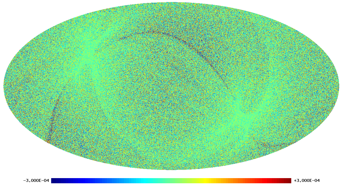
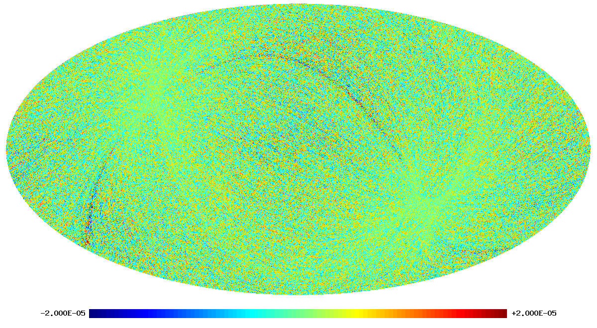
As an example, we show below images of the first realization of the 70 GHz frequency map noise for the nominal survey. The images are in order: destriped full noise, binned white noise, residual correlated noise. Note that it is difficult to see any difference between the first too images, since the residual correlated noise is more than an order of magnitude below the white noise level.

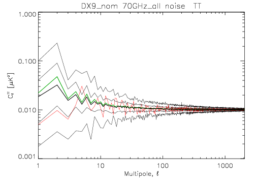
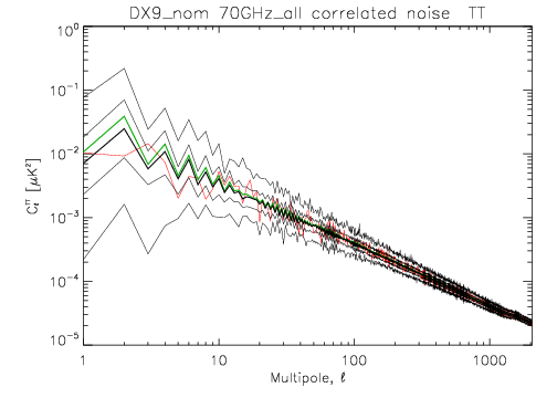
The following two images show the statistics of the angular power spectra of 101 realizations of the 70 GHz frequency map noise for the nominal survey. The thick black line shows the median $C_\ell$, and the green line the mean $C_\ell$. Thin black lines show the minimum, 16% quantile, 84% quantile, and the maximum $C_\ell$. The red line is the 102nd realization. The first plot is for the full noise in the output map, the second plot is for the residual correlated noise.