Difference between revisions of "Effective Beams"
| (84 intermediate revisions by 7 users not shown) | |||
| Line 1: | Line 1: | ||
| + | {{DISPLAYTITLE:2015 Effective Beams}} | ||
<span style="color:red"></span> | <span style="color:red"></span> | ||
==Product description== | ==Product description== | ||
| − | |||
| − | |||
The '''effective beam''' is the average of all scanning beams pointing at a certain direction within a given pixel of the sky map for a given scan strategy. It takes into account the coupling between azimuthal asymmetry of the beam and the uneven distribution of scanning angles across the sky. | The '''effective beam''' is the average of all scanning beams pointing at a certain direction within a given pixel of the sky map for a given scan strategy. It takes into account the coupling between azimuthal asymmetry of the beam and the uneven distribution of scanning angles across the sky. | ||
| − | It captures the complete information about the difference between the true and observed image of the sky. | + | It captures the complete information about the difference between the true and observed image of the sky. The effective beams are, by definition, the objects whose convolution with the true CMB sky produce the observed sky map. |
| − | |||
| − | |||
| − | |||
| − | |||
| − | |||
| − | |||
| − | |||
| − | |||
| − | |||
| − | |||
| − | |||
| − | |||
| − | |||
| − | |||
| − | |||
| − | |||
| − | |||
| − | |||
| − | |||
| − | |||
| − | |||
| − | |||
| − | |||
| − | |||
| − | |||
| − | |||
| − | |||
| − | |||
| − | |||
| − | |||
| − | |||
| − | |||
| − | |||
| − | |||
| + | Details of the beam processing are given in the respective pages for [[Beams|HFI]] and [[Beams_LFI|LFI]]. | ||
| + | The full algebra involving the effective beams for temperature and polarisation was presented in {{BibCite|mitra2010}}, and a discussion of its application to Planck data is given in the appropriate LFI {{PlanckPapers|planck2013-p02d}}, {{PlanckPapers|planck2014-a05||Planck-2015-A05}} and HFI {{PlanckPapers|planck2013-p03c}} papers. Relevant details of the processing steps are given in the [[Beams|Effective Beams]] section of this document. | ||
| − | + | <!-- Everything from here down to the "Production Process" section should eventually be moved to a new section the Joint Processing pages --> | |
| − | |||
| − | |||
| − | |||
| − | |||
===Comparison of the images of compact sources observed by Planck with FEBeCoP products=== | ===Comparison of the images of compact sources observed by Planck with FEBeCoP products=== | ||
| − | + | We show here a comparison of the FEBeCoP-derived effective beams, and associated point spread functions, PSF (the transpose of the beam matrix), to the actual images of a few compact sources observed by Planck, for all LFI and HFI frequency channels, as an example. We show below a few panels of source images organized as follows: | |
| − | We show here a comparison of the FEBeCoP derived effective beams, and associated point spread functions,PSF (the transpose of the beam matrix), to the actual images of a few compact sources observed by Planck, for all LFI and HFI frequency channels, as an example. We show below a few panels of source images organized as follows: | ||
* Row #1- DX9 images of four ERCSC objects with their galactic (l,b) coordinates shown under the color bar | * Row #1- DX9 images of four ERCSC objects with their galactic (l,b) coordinates shown under the color bar | ||
* Row #2- linear scale FEBeCoP PSFs computed using input scanning beams, Grasp Beams, GB, for LFI and B-Spline beams,BS, Mars12 apodized for the CMB channels and the BS Mars12 for the sub-mm channels, for HFI (see section Inputs below). | * Row #2- linear scale FEBeCoP PSFs computed using input scanning beams, Grasp Beams, GB, for LFI and B-Spline beams,BS, Mars12 apodized for the CMB channels and the BS Mars12 for the sub-mm channels, for HFI (see section Inputs below). | ||
* Row #3- log scale of #2; PSF iso-contours shown in solid line, elliptical Gaussian fit iso-contours shown in broken line | * Row #3- log scale of #2; PSF iso-contours shown in solid line, elliptical Gaussian fit iso-contours shown in broken line | ||
| + | <center> | ||
| − | + | <gallery widths=400px heights=400px perrow=2 caption="Comparison images of compact sources and effective beams, PSFs"> | |
| − | <gallery widths= | ||
File:30.png| '''30GHz''' | File:30.png| '''30GHz''' | ||
File:44.png| '''44GHz''' | File:44.png| '''44GHz''' | ||
| Line 69: | Line 31: | ||
File:857.png| '''857GHz''' | File:857.png| '''857GHz''' | ||
</gallery> | </gallery> | ||
| + | </center> | ||
| + | ===Histograms of the effective beam parameters=== | ||
| + | Here we present histograms of the three fit parameters - beam FWHM, ellipticity, and orientation with respect to the local meridian and of the beam solid angle. The sky is sampled (pretty sparsely) at 3072 directions which were chosen as HEALpix nside=16 pixel centers for HFI and at 768 directions which were chosen as HEALpix nside=8 pixel centers for LFI. These uniformly sample the sky. | ||
| + | Where beam solid angle is estimated according to the definition: '''<math> 4 \pi \sum</math>(effbeam)/max(effbeam)''' | ||
| + | i.e., <math> 4 \pi \sum(B_{ij}) / max(B_{ij}) </math> | ||
| + | [[File:ist_GB.png | 800px| thumb | center| '''Histograms for LFI effective beam parameters''' ]] | ||
| + | [[File:ist_BS_Mars12.png | 800px| thumb | center| '''Histograms for HFI effective beam parameters''' ]] | ||
| − | === | + | ===Sky variation of effective beams solid angle and ellipticity of the best-fit Gaussian=== |
| + | * The discontinuities at the Healpix domain edges in the maps are a visual artifact due to the interplay of the discretized effective beam and the Healpix pixel grid. | ||
| − | |||
| − | + | <gallery widths=300px heights=220px perrow=3 caption="Sky variation of effective beams ellipticity of the best-fit Gaussian"> | |
| − | + | File:e_030_GB.png| '''ellipticity - 30GHz''' | |
| + | File:e_044_GB.png| '''ellipticity - 44GHz''' | ||
| + | File:e_070_GB.png| '''ellipticity - 70GHz''' | ||
| + | File:e_100_BS_Mars12.png| '''ellipticity - 100GHz''' | ||
| + | File:e_143_BS_Mars12.png| '''ellipticity - 143GHz''' | ||
| + | File:e_217_BS_Mars12.png| '''ellipticity - 217GHz''' | ||
| + | File:e_353_BS_Mars12.png| '''ellipticity - 353GHz''' | ||
| + | File:e_545_BS_Mars12.png| '''ellipticity - 545GHz''' | ||
| + | File:e_857_BS_Mars12.png| '''ellipticity - 857GHz''' | ||
| + | </gallery> | ||
| − | + | <gallery widths=300px heights=220px perrow=3 caption="Sky (relative) variation of effective beams solid angle of the best-fit Gaussian"> | |
| − | + | File:solidarc_030_GB.png| '''beam solid angle (relative) variations wrt scanning beam - 30GHz''' | |
| + | File:solidarc_044_GB.png| '''beam solid angle (relative) variations wrt scanning beam - 44GHz''' | ||
| + | File:solidarc_070_GB.png| '''beam solid angle (relative) variations wrt scanning beam - 70GHz''' | ||
| + | File:solidarc_100_BS_Mars12.png| '''beam solid angle (relative) variations wrt scanning beam - 100GHz''' | ||
| + | File:solidarc_143_BS_Mars12.png| '''beam solid angle (relative) variations wrt scanning beam - 143GHz''' | ||
| + | File:solidarc_217_BS_Mars12.png| '''beam solid angle (relative) variations wrt scanning beam - 217GHz''' | ||
| + | File:solidarc_353_BS_Mars12.png| '''beam solid angle (relative) variations wrt scanning beam - 353GHz''' | ||
| + | File:solidarc_545_BS_Mars12.png| '''beam solid angle (relative) variations wrt scanning beam - 545GHz''' | ||
| + | File:solidarc_857_BS_Mars12.png| '''beam solid angle (relative) variations wrt scanning beam - 857GHz''' | ||
| + | </gallery> | ||
| + | <gallery widths=300px heights=220px perrow=3 caption="Sky (relative) variation of effective beams fwhm of the best-fit Gaussian"> | ||
| + | File:fwhm_030_GB.png| '''fwhm (relative) variations wrt scanning beam - 30GHz''' | ||
| + | File:fwhm_044_GB.png| '''fwhm (relative) variations wrt scanning beam - 44GHz''' | ||
| + | File:fwhm_070_GB.png| '''fwhm (relative) variations wrt scanning beam - 70GHz''' | ||
| + | File:fwhm_100_BS_Mars12.png| '''fwhm (relative) variations wrt scanning beam - 100GHz''' | ||
| + | File:fwhm_143_BS_Mars12.png| '''fwhm (relative) variations wrt scanning beam - 143GHz''' | ||
| + | File:fwhm_217_BS_Mars12.png| '''fwhm (relative) variations wrt scanning beam - 217GHz''' | ||
| + | File:fwhm_353_BS_Mars12.png| '''fwhm (relative) variations wrt scanning beam - 353GHz''' | ||
| + | File:fwhm_545_BS_Mars12.png| '''fwhm (relative) variations wrt scanning beam - 545GHz''' | ||
| + | File:fwhm_857_BS_Mars12.png| '''fwhm (relative) variations wrt scanning beam - 857GHz''' | ||
| + | </gallery> | ||
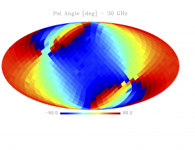
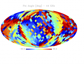
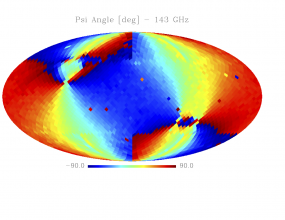
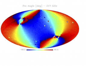
| − | ===Sky variation of effective beams | + | <gallery widths=300px heights=220px perrow=3 caption="Sky variation of effective beams <math>\psi</math> angle of the best-fit Gaussian"> |
| + | File:psi_030_GB.png| '''<math>\psi</math> - 30GHz''' | ||
| + | File:psi_044_GB.png| '''<math>\psi</math> - 44GHz''' | ||
| + | File:psi_070_GB.png| '''<math>\psi</math> - 70GHz''' | ||
| + | File:psi_100_BS_Mars12.png| '''<math>\psi</math> - 100GHz''' | ||
| + | File:psi_143_BS_Mars12.png| '''<math>\psi</math> - 143GHz''' | ||
| + | File:psi_217_BS_Mars12.png| '''<math>\psi</math> - 217GHz''' | ||
| + | File:psi_353_BS_Mars12.png| '''<math>\psi</math> - 353GHz''' | ||
| + | File:psi_545_BS_Mars12.png| '''<math>\psi</math> - 545GHz''' | ||
| + | File:psi_857_BS_Mars12.png| '''<math>\psi</math> - 857GHz''' | ||
| + | </gallery> | ||
| − | + | <!-- | |
| − | + | <gallery widths=500px heights=500px perrow=2 caption="Sky variation of effective beams solid angle and ellipticity of the best-fit Gaussian"> | |
| − | <gallery widths= | ||
File:e_030_GB.png| '''ellipticity - 30GHz''' | File:e_030_GB.png| '''ellipticity - 30GHz''' | ||
File:solidarc_030_GB.png| '''beam solid angle (relative variations wrt scanning beam - 30GHz''' | File:solidarc_030_GB.png| '''beam solid angle (relative variations wrt scanning beam - 30GHz''' | ||
| Line 98: | Line 105: | ||
File:solidarc_100_BS_Mars12.png| '''beam solid angle (relative variations wrt scanning beam - 100GHz''' | File:solidarc_100_BS_Mars12.png| '''beam solid angle (relative variations wrt scanning beam - 100GHz''' | ||
</gallery> | </gallery> | ||
| − | + | --> | |
| − | |||
| − | |||
| − | |||
===Statistics of the effective beams computed using FEBeCoP=== | ===Statistics of the effective beams computed using FEBeCoP=== | ||
| Line 141: | Line 145: | ||
====Beam solid angles for the PCCS==== | ====Beam solid angles for the PCCS==== | ||
| − | + | * <math>\Omega_{eff}</math> - is the mean beam solid angle of the effective beam, where beam solid angle is estimated according to the definition: '''<math>4 \pi \sum </math>(effbeam)/max(effbeam)''', i.e. as an integral over the full extent of the effective beam, i.e. <math> 4 \pi \sum(B_{ij}) / max(B_{ij}) </math>. | |
| − | + | * from <math>\Omega_{eff}</math> we estimate the <math>fwhm_{eff}</math>, under a Gaussian approximation - these are tabulated above | |
** <math>\Omega^{(1)}_{eff}</math> is the beam solid angle estimated up to a radius equal to one <math>fwhm_{eff}</math> and <math>\Omega^{(2)}_{eff}</math> up to a radius equal to twice the <math>fwhm_{eff}</math>. | ** <math>\Omega^{(1)}_{eff}</math> is the beam solid angle estimated up to a radius equal to one <math>fwhm_{eff}</math> and <math>\Omega^{(2)}_{eff}</math> up to a radius equal to twice the <math>fwhm_{eff}</math>. | ||
*** These were estimated according to the procedure followed in the aperture photometry code for the PCCS: if the pixel centre does not lie within the given radius it is not included (so inclusive=0 in query disc). | *** These were estimated according to the procedure followed in the aperture photometry code for the PCCS: if the pixel centre does not lie within the given radius it is not included (so inclusive=0 in query disc). | ||
| Line 170: | Line 174: | ||
| 857 || 24.244 || 0.193 || 22.646 || 0.263 || 23.985 || 0.191 | | 857 || 24.244 || 0.193 || 22.646 || 0.263 || 23.985 || 0.191 | ||
|} | |} | ||
| − | |||
==Production process== | ==Production process== | ||
| − | + | FEBeCoP, or Fast Effective Beam Convolution in Pixel space{{BibCite|mitra2010}}, is an approach to representing and computing effective beams (including both intrinsic beam shapes and the effects of scanning) that comprises the following steps: | |
| − | |||
| − | |||
| − | |||
| − | |||
| − | FEBeCoP, or Fast Effective Beam Convolution in Pixel space, is an approach to representing and computing effective beams (including both intrinsic beam shapes and the effects of scanning) that comprises the following steps: | ||
* identify the individual detectors' instantaneous optical response function (presently we use elliptical Gaussian fits of Planck beams from observations of planets; eventually, an arbitrary mathematical representation of the beam can be used on input) | * identify the individual detectors' instantaneous optical response function (presently we use elliptical Gaussian fits of Planck beams from observations of planets; eventually, an arbitrary mathematical representation of the beam can be used on input) | ||
* follow exactly the Planck scanning, and project the intrinsic beam on the sky at each actual sampling position | * follow exactly the Planck scanning, and project the intrinsic beam on the sky at each actual sampling position | ||
| Line 187: | Line 185: | ||
| − | Computation of the effective beams at each pixel for every detector is a challenging task for high resolution experiments. FEBeCoP is an efficient algorithm and implementation which enabled us to compute the pixel based effective beams using moderate computational resources. The algorithm used different mathematical and computational techniques to bring down the computation cost to a practical level, whereby several estimations of the effective beams were possible for all Planck detectors for different | + | Computation of the effective beams at each pixel for every detector is a challenging task for high resolution experiments. FEBeCoP is an efficient algorithm and implementation which enabled us to compute the pixel based effective beams using moderate computational resources. The algorithm used different mathematical and computational techniques to bring down the computation cost to a practical level, whereby several estimations of the effective beams were possible for all Planck detectors for different scan and beam models, as well as different lengths of datasets. |
===Pixel Ordered Detector Angles (PODA)=== | ===Pixel Ordered Detector Angles (PODA)=== | ||
| − | + | The main challenge in computing the effective beams is to go through the trillion samples, which gets severely limited by I/O. In the first stage, for a given dataset, ordered lists of pointing angles for each pixel - the Pixel Ordered Detector Angles (PODA) are made. This is an one-time process for each dataset. We used computers with large memory and used tedious memory management bookkeeping to make this step efficient. | |
| − | The main challenge in computing the effective beams is to go through the trillion samples, which gets severely limited by I/O. In the first stage, for a given dataset, ordered lists of pointing angles for each | ||
===effBeam=== | ===effBeam=== | ||
| − | |||
The effBeam part makes use of the precomputed PODA and unsynchronized reading from the disk to compute the beam. Here we tried to made sure that no repetition occurs in evaluating a trigonometric quantity. | The effBeam part makes use of the precomputed PODA and unsynchronized reading from the disk to compute the beam. Here we tried to made sure that no repetition occurs in evaluating a trigonometric quantity. | ||
| Line 203: | Line 199: | ||
===Computational Cost=== | ===Computational Cost=== | ||
| − | + | The computation of the effective beams has been performed at the NERSC Supercomputing Center. The table below shows the computation cost for FEBeCoP processing of the nominal mission. | |
| − | The | ||
{|border="1" cellpadding="5" cellspacing="0" align="center" style="text-align:center" | {|border="1" cellpadding="5" cellspacing="0" align="center" style="text-align:center" | ||
| − | |+ Computational cost for PODA, Effective Beam and single map convolution. | + | |+ '''Computational cost for PODA, Effective Beam and single map convolution. Wall-clock time is given as a guide, as found on the NERSC supercomputers.''' |
|- | |- | ||
|Channel ||030 || 044 || 070 || 100 || 143 || 217 || 353 || 545 || 857 | |Channel ||030 || 044 || 070 || 100 || 143 || 217 || 353 || 545 || 857 | ||
| Line 213: | Line 208: | ||
|PODA/Detector Computation time (CPU hrs) || 85 || 100 || 250 || 500 || 500 || 500 || 500 || 500 || 500 | |PODA/Detector Computation time (CPU hrs) || 85 || 100 || 250 || 500 || 500 || 500 || 500 || 500 || 500 | ||
|- | |- | ||
| − | |PODA/Detector Computation time ( | + | |PODA/Detector Computation time (wall clock hrs) || 7 || 10 || 20 || 20 || 20 || 20 || 20 || 20 || 20 |
|- | |- | ||
|Beam/Channel Computation time (CPU hrs) || 900 || 2000 || 2300 || 2800 || 3800 || 3200 || 3000 || 900 || 1100 | |Beam/Channel Computation time (CPU hrs) || 900 || 2000 || 2300 || 2800 || 3800 || 3200 || 3000 || 900 || 1100 | ||
|- | |- | ||
| − | |Beam/Channel Computation time ( | + | |Beam/Channel Computation time (wall clock hrs) || 0.5 || 0.8 || 1 || 1.5 || 2 || 1.2 || 1 || 0.5 || 0.5 |
|- | |- | ||
|Convolution Computation time (CPU hr) || 1 || 1.2 || 1.3 || 3.6 || 4.8 || 4.0 || 4.1 || 4.1 || 3.7 | |Convolution Computation time (CPU hr) || 1 || 1.2 || 1.3 || 3.6 || 4.8 || 4.0 || 4.1 || 4.1 || 3.7 | ||
|- | |- | ||
| − | |Convolution Computation time ( | + | |Convolution Computation time (wall clock sec) || 1 || 1 || 1 || 4 || 4 || 4 || 4 || 4 || 4 |
|- | |- | ||
|Effective Beam Size (GB) || 173 || 123 || 28 || 187 || 182 || 146 || 132 || 139 || 124 | |Effective Beam Size (GB) || 173 || 123 || 28 || 187 || 182 || 146 || 132 || 139 || 124 | ||
| Line 228: | Line 223: | ||
The computation cost, especially for PODA and Convolution, is heavily limited by the I/O capacity of the disc and so it depends on the overall usage of the cluster done by other users. | The computation cost, especially for PODA and Convolution, is heavily limited by the I/O capacity of the disc and so it depends on the overall usage of the cluster done by other users. | ||
| − | |||
| − | |||
==Inputs== | ==Inputs== | ||
| − | |||
| − | |||
In order to fix the convention of presentation of the scanning and effective beams, we show the classic view of the Planck focal plane as seen by the incoming CMB photon. The scan direction is marked, and the toward the center of the focal plane is at the 85 deg angle w.r.t spin axis pointing upward in the picture. | In order to fix the convention of presentation of the scanning and effective beams, we show the classic view of the Planck focal plane as seen by the incoming CMB photon. The scan direction is marked, and the toward the center of the focal plane is at the 85 deg angle w.r.t spin axis pointing upward in the picture. | ||
| − | [[File:PlanckFocalPlane.png | 500px| thumb | center| | + | [[File:PlanckFocalPlane.png | 500px| thumb | center|'''Planck Focal Plane''']] |
===The Focal Plane DataBase (FPDB)=== | ===The Focal Plane DataBase (FPDB)=== | ||
| − | + | The FPDB contains information on each detector, e.g., the orientation of the polarisation axis, different weight factors, (see the instrument [[The RIMO|RIMOs]]): | |
| − | The FPDB contains information on each detector, e.g., the orientation of the polarisation axis, different weight factors, | + | |
| + | *HFI - {{PLASingleFile|fileType=rimo|name=HFI_RIMO_R1.00.fits|link=The HFI RIMO}} | ||
| + | *LFI - {{PLASingleFile|fileType=rimo|name=LFI_RIMO_R1.12.fits|link=The LFI RIMO}} | ||
| + | |||
| + | <!-- | ||
*HFI - LFI_RIMO_DX9_PTCOR6 - {{PLASingleFile|fileType=rimo|name=HFI_RIMO_R1.00.fits|link=The HFI RIMO}} | *HFI - LFI_RIMO_DX9_PTCOR6 - {{PLASingleFile|fileType=rimo|name=HFI_RIMO_R1.00.fits|link=The HFI RIMO}} | ||
*LFI - HFI-RIMO-3_16_detilt_t2_ptcor6.fits - {{PLASingleFile|fileType=rimo|name=LFI_RIMO_R1.12.fits|link=The LFI RIMO}} | *LFI - HFI-RIMO-3_16_detilt_t2_ptcor6.fits - {{PLASingleFile|fileType=rimo|name=LFI_RIMO_R1.12.fits|link=The LFI RIMO}} | ||
| − | |||
{{PLADoc|fileType=rimo|link=The Plank RIMOS}} | {{PLADoc|fileType=rimo|link=The Plank RIMOS}} | ||
| − | + | --> | |
| − | |||
===The scanning strategy=== | ===The scanning strategy=== | ||
| − | |||
The scanning strategy, the three pointing angle for each detector for each sample: Detector pointings for the nominal mission covers about 15 months of observation from Operational Day (OD) 91 to OD 563 covering 3 surveys and half. | The scanning strategy, the three pointing angle for each detector for each sample: Detector pointings for the nominal mission covers about 15 months of observation from Operational Day (OD) 91 to OD 563 covering 3 surveys and half. | ||
===The scanbeam=== | ===The scanbeam=== | ||
| − | |||
The scanbeam modeled for each detector through the observation of planets. Which was assumed to be constant over the whole mission, though FEBeCoP could be used for a few sets of scanbeams too. | The scanbeam modeled for each detector through the observation of planets. Which was assumed to be constant over the whole mission, though FEBeCoP could be used for a few sets of scanbeams too. | ||
* LFI: [[Beams LFI#Main beams and Focalplane calibration|GRASP scanning beam]] - the scanning beams used are based on Radio Frequency Tuned Model (RFTM) smeared to simulate the in-flight optical response. | * LFI: [[Beams LFI#Main beams and Focalplane calibration|GRASP scanning beam]] - the scanning beams used are based on Radio Frequency Tuned Model (RFTM) smeared to simulate the in-flight optical response. | ||
| − | * HFI: [[ | + | * HFI: [[Beams#Scanning beams|B-Spline, BS]] based on 2 observations of Mars. |
| − | |||
| − | |||
| + | (see the instrument [[The RIMO|RIMOs]]). | ||
| + | <!-- | ||
*HFI - LFI_RIMO_DX9_PTCOR6 - {{PLASingleFile|fileType=rimo|name=HFI_RIMO_R1.00.fits|link=The HFI RIMO}} | *HFI - LFI_RIMO_DX9_PTCOR6 - {{PLASingleFile|fileType=rimo|name=HFI_RIMO_R1.00.fits|link=The HFI RIMO}} | ||
*LFI - HFI-RIMO-3_16_detilt_t2_ptcor6.fits - {{PLASingleFile|fileType=rimo|name=LFI_RIMO_R1.12.fits|link=The LFI RIMO}} | *LFI - HFI-RIMO-3_16_detilt_t2_ptcor6.fits - {{PLASingleFile|fileType=rimo|name=LFI_RIMO_R1.12.fits|link=The LFI RIMO}} | ||
[[Beams LFI#Effective beams|LFI effective beams]] | [[Beams LFI#Effective beams|LFI effective beams]] | ||
| + | --> | ||
===Beam cutoff radii=== | ===Beam cutoff radii=== | ||
| − | |||
N times geometric mean of FWHM of all detectors in a channel, where N | N times geometric mean of FWHM of all detectors in a channel, where N | ||
| Line 291: | Line 282: | ||
===Map resolution for the derived beam data object=== | ===Map resolution for the derived beam data object=== | ||
| − | |||
* <math>N_{side} = 1024 </math> for LFI frequency channels | * <math>N_{side} = 1024 </math> for LFI frequency channels | ||
* <math>N_{side} = 2048 </math> for HFI frequency channels | * <math>N_{side} = 2048 </math> for HFI frequency channels | ||
| − | |||
==Related products== | ==Related products== | ||
| − | |||
| − | |||
===Monte Carlo simulations=== | ===Monte Carlo simulations=== | ||
| Line 306: | Line 293: | ||
* generate 100 realizations of maps from a fiducial CMB power spectrum | * generate 100 realizations of maps from a fiducial CMB power spectrum | ||
* convolve each one of these maps with the effective beams using FEBeCoP | * convolve each one of these maps with the effective beams using FEBeCoP | ||
| − | * estimate the average of the Power Spectrum of each convolved realization | + | * estimate the average of the Power Spectrum of each convolved realization, and 1 <math>\sigma</math> errors |
As FEBeCoP enables fast convolutions of the input signal sky with the effective beam, thousands of simulations are generated. These Monte Carlo simulations of the signal (might it be CMB or a foreground (e.g. dust)) sky along with LevelS+Madam noise simulations were used widely for the analysis of Planck data. A suite of simulations were rendered during the mission tagged as Full Focalplane simulations, FFP#. | As FEBeCoP enables fast convolutions of the input signal sky with the effective beam, thousands of simulations are generated. These Monte Carlo simulations of the signal (might it be CMB or a foreground (e.g. dust)) sky along with LevelS+Madam noise simulations were used widely for the analysis of Planck data. A suite of simulations were rendered during the mission tagged as Full Focalplane simulations, FFP#. | ||
For example [[HL-sims#FFP6 data set|FFP6]] | For example [[HL-sims#FFP6 data set|FFP6]] | ||
| − | |||
| − | |||
===Beam Window Functions=== | ===Beam Window Functions=== | ||
| − | |||
The '''Transfer Function''' or the '''Beam Window Function''' <math> W_l </math> relates the true angular power spectra <math>C_l </math> with the observed angular power spectra <math>\widetilde{C}_l </math>: | The '''Transfer Function''' or the '''Beam Window Function''' <math> W_l </math> relates the true angular power spectra <math>C_l </math> with the observed angular power spectra <math>\widetilde{C}_l </math>: | ||
| Line 336: | Line 320: | ||
====Beam Window functions, Wl, for Planck mission==== | ====Beam Window functions, Wl, for Planck mission==== | ||
| − | + | [[File:plot_dx9_LFI_GB_pix.png | 600px | thumb | center |'''Beam Window functions, Wl, for LFI channels''']] | |
| − | + | [[File:plot_dx9_HFI_BS_M12_CMB.png | 600px | thumb | |center |'''Beam Window functions, Wl, for HFI channels''']] | |
| − | |||
| − | [[File:plot_dx9_LFI_GB_pix.png | | ||
| − | [[File:plot_dx9_HFI_BS_M12_CMB.png | | ||
| − | |||
| − | |||
| − | |||
==File Names== | ==File Names== | ||
| − | --- | + | The effective beams are provided by the PLA as FITS files containg HEALPix maps of the beams. For the file names the following convention is used: |
| + | *Single beam query: '''beams_FFF_''PixelNumber''.fits''' | ||
| + | **FFF is the channel frequency (one of '''30''', '''44''', '''70''', '''100''', '''143''', '''217''', '''353''', '''545''', '''857'''); | ||
| + | ** ''PixelNumber'' is the number of the pixel to which the beam corresponds (<math>0</math> - <math>12 \times N_{\rm side}^2 - 1</math>). For the LFI <math>N_{\rm side}=1024</math>, for the HFI <math>N_{\rm side}=2048</math>; | ||
| + | *Multiple beam query: '''beams_FFF_''FirstPixelNumber''-''LastPixelNumber''.zip''' <br /> The compressed files contains a set of files with the beams for the pixels covereing the selected region. FFF as for sinle beam query. The naming convention for the beam files contained in the ''.zip'' file is the same as for single beam queries. | ||
| + | ** ''FirstPixelNumber'' is the lowest pixel number for the area covered by the request; | ||
| + | ** ''LastPixelNumber'' is the highest pixel number for the area covered by the request; | ||
| − | + | ==File format== | |
| + | The FITS files provided by the PLA contain HEALPix maps of the beams. | ||
| − | + | == References == | |
| − | + | <References /> | |
| − | |||
| − | |||
| − | |||
| − | |||
| − | |||
| − | |||
| − | |||
| − | |||
| − | |||
| − | |||
| − | |||
| − | |||
| − | |||
| − | |||
| − | |||
| − | |||
| − | |||
| − | |||
| − | |||
| − | |||
| − | |||
| − | |||
| − | |||
| − | |||
| − | [[Category:Mission | + | [[Category:Mission products|004]] |
Latest revision as of 10:37, 5 February 2015
Contents
- 1 Product description
- 2 Production process
- 3 Inputs
- 4 Related products
- 5 File Names
- 6 File format
- 7 References
Product description[edit]
The effective beam is the average of all scanning beams pointing at a certain direction within a given pixel of the sky map for a given scan strategy. It takes into account the coupling between azimuthal asymmetry of the beam and the uneven distribution of scanning angles across the sky. It captures the complete information about the difference between the true and observed image of the sky. The effective beams are, by definition, the objects whose convolution with the true CMB sky produce the observed sky map.
Details of the beam processing are given in the respective pages for HFI and LFI.
The full algebra involving the effective beams for temperature and polarisation was presented in [1], and a discussion of its application to Planck data is given in the appropriate LFI Planck-2013-IV[2], Planck-2015-A05[3] and HFI Planck-2013-VII[4] papers. Relevant details of the processing steps are given in the Effective Beams section of this document.
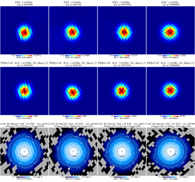
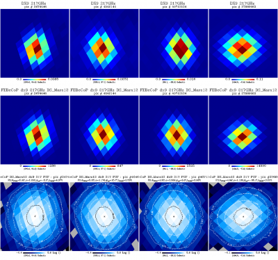
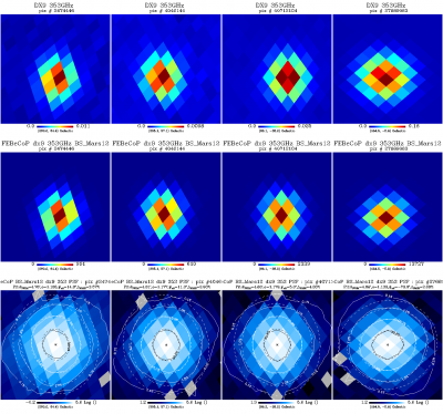
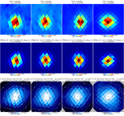
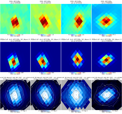
Comparison of the images of compact sources observed by Planck with FEBeCoP products[edit]
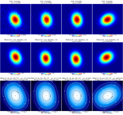
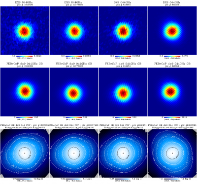
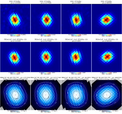
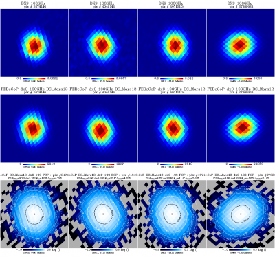
We show here a comparison of the FEBeCoP-derived effective beams, and associated point spread functions, PSF (the transpose of the beam matrix), to the actual images of a few compact sources observed by Planck, for all LFI and HFI frequency channels, as an example. We show below a few panels of source images organized as follows:
- Row #1- DX9 images of four ERCSC objects with their galactic (l,b) coordinates shown under the color bar
- Row #2- linear scale FEBeCoP PSFs computed using input scanning beams, Grasp Beams, GB, for LFI and B-Spline beams,BS, Mars12 apodized for the CMB channels and the BS Mars12 for the sub-mm channels, for HFI (see section Inputs below).
- Row #3- log scale of #2; PSF iso-contours shown in solid line, elliptical Gaussian fit iso-contours shown in broken line
- Comparison images of compact sources and effective beams, PSFs
30GHz
44GHz
70GHz
100GHz
143GHz
217GHz
353GHz
545GHz
857GHz


Histograms of the effective beam parameters[edit]
Here we present histograms of the three fit parameters - beam FWHM, ellipticity, and orientation with respect to the local meridian and of the beam solid angle. The sky is sampled (pretty sparsely) at 3072 directions which were chosen as HEALpix nside=16 pixel centers for HFI and at 768 directions which were chosen as HEALpix nside=8 pixel centers for LFI. These uniformly sample the sky.
Where beam solid angle is estimated according to the definition: (effbeam)/max(effbeam) i.e.,


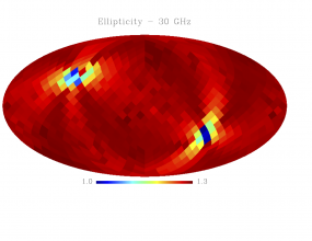
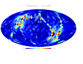
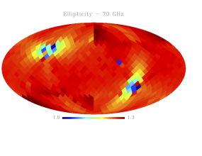
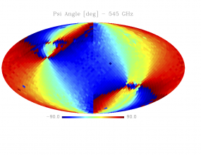
Sky variation of effective beams solid angle and ellipticity of the best-fit Gaussian[edit]
- The discontinuities at the Healpix domain edges in the maps are a visual artifact due to the interplay of the discretized effective beam and the Healpix pixel grid.
- Sky variation of effective beams ellipticity of the best-fit Gaussian
ellipticity - 30GHz
ellipticity - 44GHz
ellipticity - 70GHz
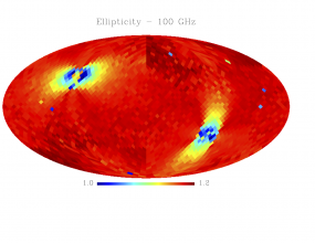
ellipticity - 100GHz
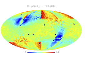
ellipticity - 143GHz
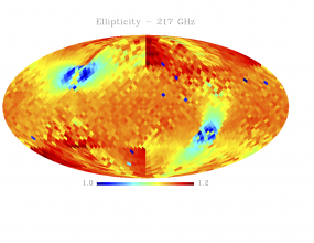
ellipticity - 217GHz
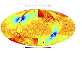
ellipticity - 353GHz
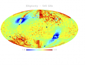
ellipticity - 545GHz
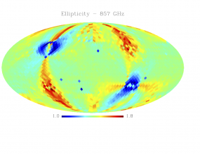
ellipticity - 857GHz


- Sky (relative) variation of effective beams solid angle of the best-fit Gaussian
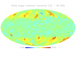
beam solid angle (relative) variations wrt scanning beam - 30GHz
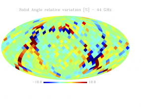
beam solid angle (relative) variations wrt scanning beam - 44GHz
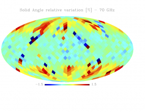
beam solid angle (relative) variations wrt scanning beam - 70GHz
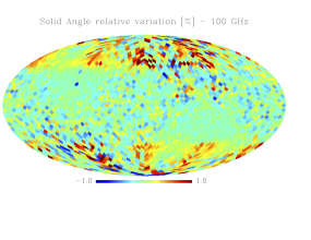
beam solid angle (relative) variations wrt scanning beam - 100GHz
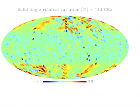
beam solid angle (relative) variations wrt scanning beam - 143GHz
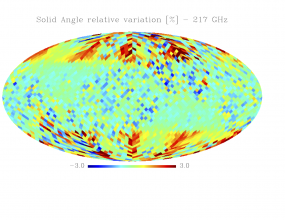
beam solid angle (relative) variations wrt scanning beam - 217GHz
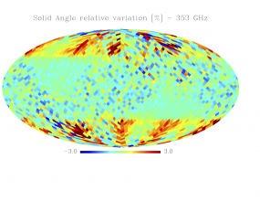
beam solid angle (relative) variations wrt scanning beam - 353GHz
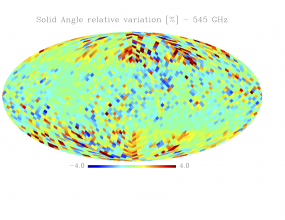
beam solid angle (relative) variations wrt scanning beam - 545GHz
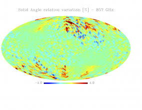
beam solid angle (relative) variations wrt scanning beam - 857GHz


- Sky (relative) variation of effective beams fwhm of the best-fit Gaussian
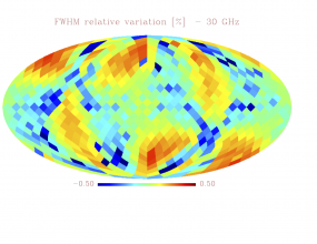
fwhm (relative) variations wrt scanning beam - 30GHz
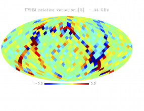
fwhm (relative) variations wrt scanning beam - 44GHz
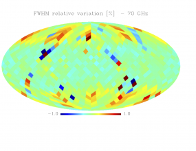
fwhm (relative) variations wrt scanning beam - 70GHz
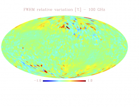
fwhm (relative) variations wrt scanning beam - 100GHz
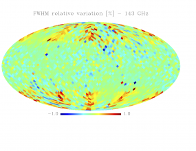
fwhm (relative) variations wrt scanning beam - 143GHz
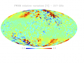
fwhm (relative) variations wrt scanning beam - 217GHz
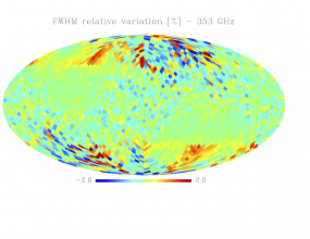
fwhm (relative) variations wrt scanning beam - 353GHz
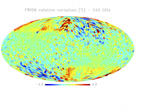
fwhm (relative) variations wrt scanning beam - 545GHz
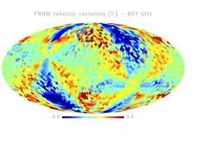
fwhm (relative) variations wrt scanning beam - 857GHz


- Sky variation of effective beams <math
- 30GHz
- 44GHz

- 70GHz

- 100GHz
- 143GHz
- 217GHz

- 353GHz
- 545GHz

- 857GHz


Statistics of the effective beams computed using FEBeCoP[edit]
We tabulate the simple statistics of FWHM, ellipticity (e), orientation () and beam solid angle, (), for a sample of 3072 and 768 directions on the sky for HFI and LFI data respectively. Statistics shown in the Table are derived from the histograms shown above.
- The derived beam parameters are representative of the DPC NSIDE 1024 and 2048 healpix maps (they include the pixel window function).
- The reported FWHM_eff are derived from the beam solid angles, under a Gaussian approximation. These are best used for flux determination while the the Gaussian fits to the effective beam maps are more suited for source identification.
| frequency | mean(fwhm) [arcmin] | sd(fwhm) [arcmin] | mean(e) | sd(e) | mean() [degree] | sd() [degree] | mean() [arcmin] | sd() [arcmin] | FWHM_eff [arcmin] |
|---|---|---|---|---|---|---|---|---|---|
| 030 | 32.239 | 0.013 | 1.320 | 0.031 | -0.304 | 55.349 | 1189.513 | 0.842 | 32.34 |
| 044 | 27.005 | 0.552 | 1.034 | 0.033 | 0.059 | 53.767 | 832.946 | 31.774 | 27.12 |
| 070 | 13.252 | 0.033 | 1.223 | 0.026 | 0.587 | 55.066 | 200.742 | 1.027 | 13.31 |
| 100 | 9.651 | 0.014 | 1.186 | 0.023 | -0.024 | 55.400 | 105.778 | 0.311 | 9.66 |
| 143 | 7.248 | 0.015 | 1.036 | 0.009 | 0.383 | 54.130 | 59.954 | 0.246 | 7.27 |
| 217 | 4.990 | 0.025 | 1.177 | 0.030 | 0.836 | 54.999 | 28.447 | 0.271 | 5.01 |
| 353 | 4.818 | 0.024 | 1.147 | 0.028 | 0.655 | 54.745 | 26.714 | 0.250 | 4.86 |
| 545 | 4.682 | 0.044 | 1.161 | 0.036 | 0.544 | 54.876 | 26.535 | 0.339 | 4.84 |
| 857 | 4.325 | 0.055 | 1.393 | 0.076 | 0.876 | 54.779 | 24.244 | 0.193 | 4.63 |
Beam solid angles for the PCCS[edit]
- - is the mean beam solid angle of the effective beam, where beam solid angle is estimated according to the definition: (effbeam)/max(effbeam), i.e. as an integral over the full extent of the effective beam, i.e. .
- from we estimate the , under a Gaussian approximation - these are tabulated above
- is the beam solid angle estimated up to a radius equal to one and up to a radius equal to twice the .
- These were estimated according to the procedure followed in the aperture photometry code for the PCCS: if the pixel centre does not lie within the given radius it is not included (so inclusive=0 in query disc).
- is the beam solid angle estimated up to a radius equal to one and up to a radius equal to twice the .
| Band | [arcmin] | spatial variation [arcmin] | [arcmin] | spatial variation-1 [arcmin] | [arcmin] | spatial variation-2 [arcmin] |
| 30 | 1189.513 | 0.842 | 1116.494 | 2.274 | 1188.945 | 0.847 |
| 44 | 832.946 | 31.774 | 758.684 | 29.701 | 832.168 | 31.811 |
| 70 | 200.742 | 1.027 | 186.260 | 2.300 | 200.591 | 1.027 |
| 100 | 105.778 | 0.311 | 100.830 | 0.410 | 105.777 | 0.311 |
| 143 | 59.954 | 0.246 | 56.811 | 0.419 | 59.952 | 0.246 |
| 217 | 28.447 | 0.271 | 26.442 | 0.537 | 28.426 | 0.271 |
| 353 | 26.714 | 0.250 | 24.827 | 0.435 | 26.653 | 0.250 |
| 545 | 26.535 | 0.339 | 24.287 | 0.455 | 26.302 | 0.337 |
| 857 | 24.244 | 0.193 | 22.646 | 0.263 | 23.985 | 0.191 |
Production process[edit]
FEBeCoP, or Fast Effective Beam Convolution in Pixel space[1], is an approach to representing and computing effective beams (including both intrinsic beam shapes and the effects of scanning) that comprises the following steps:
- identify the individual detectors' instantaneous optical response function (presently we use elliptical Gaussian fits of Planck beams from observations of planets; eventually, an arbitrary mathematical representation of the beam can be used on input)
- follow exactly the Planck scanning, and project the intrinsic beam on the sky at each actual sampling position
- project instantaneous beams onto the pixelized map over a small region (typically <2.5 FWHM diameter)
- add up all beams that cross the same pixel and its vicinity over the observing period of interest
- create a data object of all beams pointed at all N'_pix_' directions of pixels in the map at a resolution at which this precomputation was executed (dimension N'_pix_' x a few hundred)
- use the resulting beam object for very fast convolution of all sky signals with the effective optical response of the observing mission
Computation of the effective beams at each pixel for every detector is a challenging task for high resolution experiments. FEBeCoP is an efficient algorithm and implementation which enabled us to compute the pixel based effective beams using moderate computational resources. The algorithm used different mathematical and computational techniques to bring down the computation cost to a practical level, whereby several estimations of the effective beams were possible for all Planck detectors for different scan and beam models, as well as different lengths of datasets.
Pixel Ordered Detector Angles (PODA)[edit]
The main challenge in computing the effective beams is to go through the trillion samples, which gets severely limited by I/O. In the first stage, for a given dataset, ordered lists of pointing angles for each pixel - the Pixel Ordered Detector Angles (PODA) are made. This is an one-time process for each dataset. We used computers with large memory and used tedious memory management bookkeeping to make this step efficient.
effBeam[edit]
The effBeam part makes use of the precomputed PODA and unsynchronized reading from the disk to compute the beam. Here we tried to made sure that no repetition occurs in evaluating a trigonometric quantity.
One important reason for separating the two steps is that they use different schemes of parallel computing. The PODA part requires parallelisation over time-order-data samples, while the effBeam part requires distribution of pixels among different computers.
Computational Cost[edit]
The computation of the effective beams has been performed at the NERSC Supercomputing Center. The table below shows the computation cost for FEBeCoP processing of the nominal mission.
| Channel | 030 | 044 | 070 | 100 | 143 | 217 | 353 | 545 | 857 |
| PODA/Detector Computation time (CPU hrs) | 85 | 100 | 250 | 500 | 500 | 500 | 500 | 500 | 500 |
| PODA/Detector Computation time (wall clock hrs) | 7 | 10 | 20 | 20 | 20 | 20 | 20 | 20 | 20 |
| Beam/Channel Computation time (CPU hrs) | 900 | 2000 | 2300 | 2800 | 3800 | 3200 | 3000 | 900 | 1100 |
| Beam/Channel Computation time (wall clock hrs) | 0.5 | 0.8 | 1 | 1.5 | 2 | 1.2 | 1 | 0.5 | 0.5 |
| Convolution Computation time (CPU hr) | 1 | 1.2 | 1.3 | 3.6 | 4.8 | 4.0 | 4.1 | 4.1 | 3.7 |
| Convolution Computation time (wall clock sec) | 1 | 1 | 1 | 4 | 4 | 4 | 4 | 4 | 4 |
| Effective Beam Size (GB) | 173 | 123 | 28 | 187 | 182 | 146 | 132 | 139 | 124 |
The computation cost, especially for PODA and Convolution, is heavily limited by the I/O capacity of the disc and so it depends on the overall usage of the cluster done by other users.
Inputs[edit]
In order to fix the convention of presentation of the scanning and effective beams, we show the classic view of the Planck focal plane as seen by the incoming CMB photon. The scan direction is marked, and the toward the center of the focal plane is at the 85 deg angle w.r.t spin axis pointing upward in the picture.

The Focal Plane DataBase (FPDB)[edit]
The FPDB contains information on each detector, e.g., the orientation of the polarisation axis, different weight factors, (see the instrument RIMOs):
- HFI - The HFI RIMO
- LFI - The LFI RIMO
The scanning strategy[edit]
The scanning strategy, the three pointing angle for each detector for each sample: Detector pointings for the nominal mission covers about 15 months of observation from Operational Day (OD) 91 to OD 563 covering 3 surveys and half.
The scanbeam[edit]
The scanbeam modeled for each detector through the observation of planets. Which was assumed to be constant over the whole mission, though FEBeCoP could be used for a few sets of scanbeams too.
- LFI: GRASP scanning beam - the scanning beams used are based on Radio Frequency Tuned Model (RFTM) smeared to simulate the in-flight optical response.
- HFI: B-Spline, BS based on 2 observations of Mars.
(see the instrument RIMOs).
Beam cutoff radii[edit]
N times geometric mean of FWHM of all detectors in a channel, where N
| channel | Cutoff Radii in units of fwhm | fwhm of full beam extent |
| 30 - 44 - 70 | 2.5 | |
| 100 | 2.25 | 23.703699 |
| 143 | 3 | 21.057402 |
| 217-353 | 4 | 18.782754 |
| sub-mm | 4 | 18.327635(545GHz) ; 17.093706(857GHz) |
Map resolution for the derived beam data object[edit]
- for LFI frequency channels
- for HFI frequency channels
Related products[edit]
Monte Carlo simulations[edit]
FEBeCoP software enables fast, full-sky convolutions of the sky signals with the Effective beams in pixel domain. Hence, a large number of Monte Carlo simulations of the sky signal maps map convolved with realistically rendered, spatially varying, asymmetric Planck beams can be easily generated. We performed the following steps:
- generate the effective beams with FEBeCoP for all frequencies for dDX9 data and Nominal Mission
- generate 100 realizations of maps from a fiducial CMB power spectrum
- convolve each one of these maps with the effective beams using FEBeCoP
- estimate the average of the Power Spectrum of each convolved realization, and 1 errors
As FEBeCoP enables fast convolutions of the input signal sky with the effective beam, thousands of simulations are generated. These Monte Carlo simulations of the signal (might it be CMB or a foreground (e.g. dust)) sky along with LevelS+Madam noise simulations were used widely for the analysis of Planck data. A suite of simulations were rendered during the mission tagged as Full Focalplane simulations, FFP#.
For example FFP6
Beam Window Functions[edit]
The Transfer Function or the Beam Window Function relates the true angular power spectra with the observed angular power spectra :
Note that, the window function can contain a pixel window function (depending on the definition) and it is {\em not the angular power spectra of the scanbeams}, though, in principle, one may be able to connect them though fairly complicated algebra.
The window functions are estimated by performing Monte-Carlo simulations. We generate several random realisations of the CMB sky starting from a given fiducial , convolve the maps with the pre-computed effective beams, compute the convolved power spectra , divide by the power spectra of the unconvolved map and average over their ratio. Thus, the estimated window function
For subtle reasons, we perform a more rigorous estimation of the window function by comparing C^{conv}_l with convolved power spectra of the input maps convolved with a symmetric Gaussian beam of comparable (but need not be exact) size and then scaling the estimated window function accordingly.
Beam window functions are provided in the RIMO.
Beam Window functions, Wl, for Planck mission[edit]


File Names[edit]
The effective beams are provided by the PLA as FITS files containg HEALPix maps of the beams. For the file names the following convention is used:
- Single beam query: beams_FFF_PixelNumber.fits
- FFF is the channel frequency (one of 30, 44, 70, 100, 143, 217, 353, 545, 857);
- PixelNumber is the number of the pixel to which the beam corresponds ( - ). For the LFI , for the HFI ;
- Multiple beam query: beams_FFF_FirstPixelNumber-LastPixelNumber.zip
The compressed files contains a set of files with the beams for the pixels covereing the selected region. FFF as for sinle beam query. The naming convention for the beam files contained in the .zip file is the same as for single beam queries.- FirstPixelNumber is the lowest pixel number for the area covered by the request;
- LastPixelNumber is the highest pixel number for the area covered by the request;
File format[edit]
The FITS files provided by the PLA contain HEALPix maps of the beams.
References[edit]
- ↑ 1.01.1 Fast Pixel Space Convolution for Cosmic Microwave Background Surveys with Asymmetric Beams and Complex Scan Strategies: FEBeCoP, S. Mitra, G. Rocha, K. M. Górski, K. M. Huffenberger, H. K. Eriksen, M. A. J. Ashdown, C. R. Lawrence, ApJS, 193, 5-+, (2011).
- ↑ Planck 2013 results. IV. Low Frequency Instrument beams and window functions, Planck Collaboration, 2014, A&A, 571, A4
- ↑ Planck 2015 results. IV. LFI beams and window functions, Planck Collaboration, 2016, A&A, 594, A4.
- ↑ Planck 2013 results. VII. HFI time response and beams, Planck Collaboration, 2014, A&A, 571, A7
Cosmic Microwave background
(Planck) Low Frequency Instrument
(Planck) High Frequency Instrument
Early Release Compact Source Catalog
Full-Width-at-Half-Maximum
Data Processing Center
Operation Day definition is geometric visibility driven as it runs from the start of a DTCP (satellite Acquisition Of Signal) to the start of the next DTCP. Given the different ground stations and spacecraft will takes which station for how long, the OD duration varies but it is basically once a day.
Planck Legacy Archive
Flexible Image Transfer Specification
(Hierarchical Equal Area isoLatitude Pixelation of a sphere, <ref name="Template:Gorski2005">HEALPix: A Framework for High-Resolution Discretization and Fast Analysis of Data Distributed on the Sphere, K. M. Górski, E. Hivon, A. J. Banday, B. D. Wandelt, F. K. Hansen, M. Reinecke, M. Bartelmann, ApJ, 622, 759-771, (2005).