Internal overall validation

Overview

Data validation is a step of paramount importance in the complex process of data analysis and the extraction of the final scientific goals of an experiment. The LFI approach to data validation is based upon null-tests approach and here we present the rationale behind envisaged/performed null-tests and the actual results for the present data release. Also we will provide results of the same kind of tests performed on previous release to show the overall improvements in the data quality.

Null-tests approach

In general null-tests are performed in order to highlight possible issues in the data related to instrumental systematic effect not properly accounted for within the processing pipeline and related to known events of the operational conditions (e.g. switch-over of the sorption coolers) or to intrinsic instrument properties coupled with sky signal like stray-light contamination.

Such null-tests are expected to be performed considering data on different time scales ranging from 1-minute to one year of observations, at different unit level (radiometer, horn, horn-pair, within frequency and cross-frequency both in total intensity and, when applicable, to polarisation.

This is quite demanding in terms of all possible combinations. In addition some tools are already available and can be properly used for this kind of analysis. However it may be possible that on some specific time-scale, detailed tools have to be developed in order to produce the desired null-test results. In this respect the actual half-ring jack-knives are suitable to track any effects on pointing period times scales. On time-scales between half-ring and survey there are lot of possibilities. It has to be verified if the actual code producing half-ring jack-knives (madam) can handle data producing jack-knives of larger (e.g. 1 hour) times scales.

It is fundamental that such test have to be performed on DPC data product with clear and identified properties (e.g. single [math]R[/math], gains, single fit, etc.) in order to avoid any possible mis-understanding due to usage of non homogeneous data sets.

Many of the null-tests proposed are done at map level with sometime compression of their statistical information into an angular power spectrum. However together with full-sky maps it is interesting to have a closer look on some specific sources. I would be important to compare fluxes from both polarized and un-polarized point sources with different radiometers in order to asses possible calibration mis-match and/or polarization leakage issues. Such comparison will also possibly indicate problems related to channel central frequencies. The proposed set of sources would be: M42, Tau A, Cas A and Cyg A. However other [math]H \, II[/math] regions like Perseus are valuable. One can compare directly their fluxes from different sky surveys and/or the flux of the difference map and how this is consistent with instrumental noise.

Which kind of effect is probed with a null-test on a specific time scale? Here it is a simple list. At survey time scale it is possible to underlying any side-lobes effects, while on time scales of full-mission, it is possible to have an indication of calibration problems when observing the sky with the same S/C orientation. Differences at this time scale between horns at the same frequency may also reveal central frequency and beam issues.

Total Intensity Null Tests

In order to highlight different issues, several time scales and data combinations are considered. The following table is a sort of null-test matrix to be filled with test results. It should be important to try to set a sort of pass/fail criteria for each of the tests and to be prepared to detailed actions in order to avoid and correct any failure of the tests. To assess the results an idea could be to proceed as in the nominal pipeline i.e. to compare the angular power spectra of null test maps with a fiducial angular power spectrum of a white noise map. This could be made automatic and, in case the test does not pass then a more thorough investigation could be performed. This will provide an overall indication of the residuals. However structures in the residual are important as well as the overall average level and visual inspection of the data is therefore fundamental.

Concerning null-tests on various time scales a comment is in order. At large time scales (i.e. of the order of a survey or more) it is clear that the basic data set will be made of the single survey maps at radiometer/horn/frequency level that will be properly combined to obtain the null-test under consideration. For example at 6 months time scale we will analysis maps of the difference between different surveys for the radiometer/horn/frequency under test. On the other hand at 12 months time scale we will combine surveys 1 and 2 together to be compared with the same combination for surveys 3 and 4. At full-mission time scale, the analysis it is not always possible e.g. at radiometer level we have only one full-mission data set. However it would be interesting to combine odd surveys together and compare them with even surveys again combined together. On shorter time scales (i.e. less than a survey) the data products to be considered are different and will be the output of the jack-knives code when different time scales are considered: the usual half-ring JK on pointing period time scale and the new, if possible, jack-knives on 1 minute time scale. Therefore null-tests will use both surveys/full-mission maps as well as tailored jack-knives maps.

The following table reports our total intensity null-tests matrix with a [math]\checkmark[/math] where tests are possible.

Data Set	1minute	1 hour	Survey	Full Mission
Radiometer (M/S)	[math]\checkmark[/math]	[math]\checkmark[/math]	[math]\checkmark[/math]	[math]\checkmark[/math]
Horn (M+S)	[math]\checkmark[/math]	[math]\checkmark[/math]	[math]\checkmark[/math]	[math]\checkmark[/math]
Horn Pair[math]^1[/math]			[math]\checkmark[/math]	[math]\checkmark[/math]
Frequency	[math]\checkmark[/math]	[math]\checkmark[/math]	[math]\checkmark[/math]	[math]\checkmark[/math]
Cross-Frequency			[math]\checkmark[/math]	[math]\checkmark[/math]

[math]^1[/math] this is [math](M+S)/2[/math] and differences are between couple of horns (e.g. (28M+28S)/2- (27M+27S)/2)

Polarisation Null Tests

The same arguments applies also for polarization analysis with only some differences regarding the possible combination producing polarized data. Radiometer will not be available, instead of sum between M and S radiometer we will consider their difference.

Data Set	1minute	1 hour	Survey	Full Mission
Horn (M-S)	[math]\checkmark[/math]	[math]\checkmark[/math]	[math]\checkmark[/math]	[math]\checkmark[/math]
Horn Pair[math]^1[/math]			[math]\checkmark[/math]	[math]\checkmark[/math]
Frequency	[math]\checkmark[/math]	[math]\checkmark[/math]	[math]\checkmark[/math]	[math]\checkmark[/math]
Cross-Frequency			[math]\checkmark[/math]	[math]\checkmark[/math]

[math]^1[/math] this is difference between couple of horns (e.g. (28M-28S)/2- (27M-27S)/2)

Practical Considerations

For practical purposed and visual inspection of the null-tests results it would be useful to produce results smoothed at [math]3^\circ[/math] (and at [math]10^\circ[/math] for highlight larger angular scales) for all the total intensity maps. For polarization, as we already did several times when comparing to [math]WMAP[/math] data, a downgrade of the product at [math]N_{\rm side}=128[/math] would be useful to highlight large scale residuals. These considerations are free to evolve according to our needs.

Due to large possibilities and number of data sets to be considered, it would be desirable to have sort of automatic tools that ingest two, or more, inputs maps and produce difference map(s) and corresponding angular power spectrum(spectra). This has been implemented using Python language and interacting directly with FITS files of a specific data release. The code is parallel and can run both at NERSC and at DPC producing consistent results. In addition for each null-tests performed a JSON DB file is produced in which main test informations are stored together with interesting computed quantities like mean, standard deviation of the residual maps. Beside JSON files also GIF images of the null-test are produced. Such JSON and GIF files are used to create (both with Python again and with Scheme) a report in form of an HTML page from the LFI Wiki.

Together with images, power spectra of the residual are also produced and compared with the expected level of white noise derived from the half-ring jack-knifes. With these quantities are combined to produce a sort of [math]\chi^2[/math]. This gives an indication of the deviation of the residuals with respect to the white noise level. Of course underlying signal does not posses a Gaussian statistic and therefore with non-Gaussian data, the [math]\chi^2[/math] tests is less meaningful. However this gives an hint on the presence of residuals which in some cases are indeed expected: in fact making difference between odd and even survey at horn and frequency level, is a way to show the signature of the external stray-light which, although properly accounted for during the calibration procedure, has not been removed from the data.

Consistency checks

All the details can be found in Planck-2013-IIPlanck-2015-A03.

Intra frequency consistency check

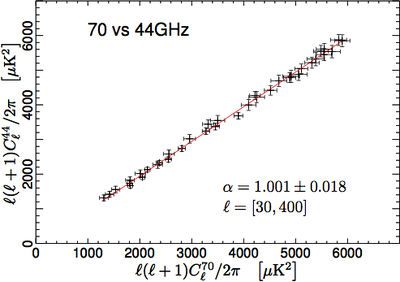
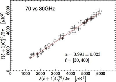
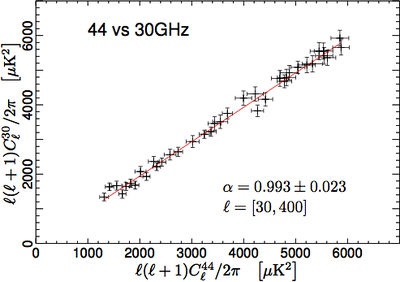
We have tested the consistency between 30, 44, and 70 GHz maps by comparing the power spectra in the multipole range around the first acoustic peak. In order to do so, we have removed the estimated contribution from unresolved point source from the spectra. We have then built the scatter plots for the three frequency pairs, i.e. 70 vs 30 GHz, 70 vs 44 GHz, and 44 vs 30 GHz, and performed a linear fit accounting for errors on both axis. The results reported in Fig. 1 show that the three power spectra are consistent within the errors. Moreover, please note that current error budget does not account for foreground removal, calibration, and window function uncertainties. Hence, the resulting agreement between spectra at different frequencies can be fairly considered even more significant.

Figure 1. Consistency between spectral estimates at different frequencies. From top to bottom: 70 vs 44 GHz; 70 vs 30 GHz; 44 vs 30 GHz. Solid red lines are the best fit of the linear regressions, whose angular coefficients [math]\alpha[/math] are consistent with 1 within the errors.

70 GHz internal consistency check

We use the Hausman test to assess the consistency of auto and cross spectral estimates at 70 GHz. We define the statistic:

[math] H_{\ell}=\left(\hat{C_{\ell}}-\tilde{C_{\ell}}\right)/\sqrt{Var\left\{ \hat{C_{\ell}}-\tilde{C_{\ell}}\right\} } [/math]

where [math]\hat{C_{\ell}}[/math] and [math]\tilde{C_{\ell}}[/math] represent auto- and cross-spectra respectively. In order to combine information from different multipoles into a single quantity, we define the following quantity:

[math] B_{L}(r)=\frac{1}{\sqrt{L}}\sum_{\ell=2}^{[Lr]}H_{\ell},r\in\left[0,1\right] [/math]

where [math][.][/math] denotes integer part. The distribution of [math]B_{L}(r)[/math] converges (in a functional sense) to a Brownian motion process, which can be studied through the statistics [math]s_{1}=\textrm{sup}_{r}B_{L}(r)[/math] [math]s_{2}=\textrm{sup}_{r}|B_{L}(r)|[/math] and [math]s_{3}=\int_{0}^{1}B_{L}^{2}(r)dr[/math]. Using the FFP7 simulations we derive the empirical distribution for all the three test statistics and we compare with results obtained from Planck data (see Fig. 2). Thus, the Hausman test shows no statistically significant inconsistencies between the two spectral estimates.

Figure 2. From left to right, the empirical distribution (estimated via FFP7) of the [math]s_{1},s_{2},s_{3}[/math] statistics (see text). The vertical line represents 70 GHz data.

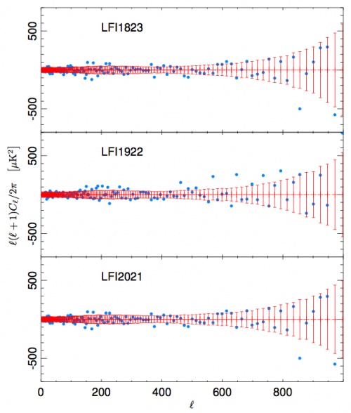
As a further test, we have estimated the temperature power spectrum for each of three horn-pair map, and we have compared the results with the spectrum obtained from all the 12 radiometers shown above. In Fig. 3 we show the difference between the horn-pair and the combined power spectra. Again, the error bars have been estimated from the FFP7 simulated dataset. A [math]\chi^{2}[/math] analysis of the residual shows that they are compatible with the null hypothesis, confirming the strong consistency of the estimates.

Figure 3. Residuals between the auto power spectra of the horn pair maps and the power spectrum of the full 70 GHz frequency map. Error bars are derived from FFP7 simulations.