CMB spectrum & Likelihood Code

2015 CMB spectra

General description

TT

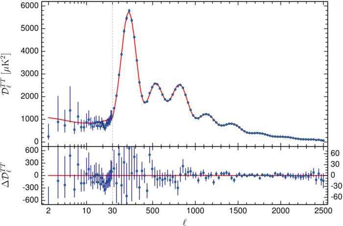
The Planck best-fit CMB temperature power spectrum, shown in the figure below, covers the wide range of multipoles [math] \ell [/math] = 2-2508. Over the multipole range [math] \ell [/math] = 2–29, the power spectrum is derived from the Commander: component separation algorithm applied to the combination of Planck 2015 temperature data between 30 and 857 GHz, the 9-year WMAP sky maps, and the 408 MHz Haslam et al. (1982) survey, including 93% of the sky Planck-2015-A10 . The asymmetric error bars associated to this spectrum are the 68% confidence limits and include the uncertainties due to foreground subtraction.

For multipoles equal or greater than [math]\ell=30[/math], instead, the spectrum is derived from the Plik likelihood Planck-2015-A11 by optimally combining the spectra in the frequency range 100-217 GHz, and correcting them for unresolved foregrounds using the best-fit foreground solution from a Planck TT+lowP [math]\Lambda[/math]CDM run. Associated 1-sigma errors include beam uncertainties. Both Commander and Plik are described in more details in the sections below.

The Planck 2015 TT power spectrum. Logarithmic x-scale up to [math]\ell = 30 [/math] , linear at higher [math]\ell[/math]. The red line is the Planck best-fit primordial power spectrum (cf Planck TT+lowP in Table 3 of Planck-2015-A15[3]). Residuals with respect to this model are shown in the lower panel. The error bars show [math]\pm 1\sigma[/math] uncertainties.

TE and EE

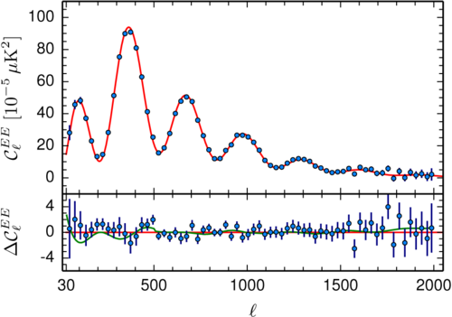
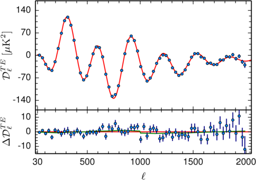
The Planck best-fit CMB polarization and temperature-polarization cross-correlation power spectra, shown in the figure below, cover the multipole range [math] \ell [/math] = 30-1996. The data points relative to the multipole range [math] \ell [/math] = 2-29 will be released at a later time. Analogously to the TT case, the [math] \ell\ge 30 [/math] spectrum is derived from the Plik likelihood Planck-2015-A11 by optimally combining the spectra in the frequency range 100-217 GHz, and correcting them for unresolved foregrounds using the best-fit foreground solution from a Planck TT,TE,EE+lowP [math]\Lambda[/math]CDM run.

The Planck 2015 EE power spectrum. The red line is the Planck best-fit primordial power spectrum (cf Planck TT+lowP in Table 3 of Planck-2015-A15). Residuals with respect to this model are shown in the lower panel. The error bars show [math]\pm 1\sigma[/math] uncertainties. The green lines in the lower panels show the best-fit temperature-to-polarization leakage model of Eqs. (11a) and (11b) in Planck-2015-A15.

The Planck 2015 TE power spectrum. The red line is the Planck best-fit primordial power spectrum (cf Planck TT+lowP in Table 3 of Planck-2015-A15). Residuals with respect to this model are shown in the lower panel. The error bars show [math]\pm 1\sigma[/math] uncertainties. The green lines in the lower panels show the best-fit temperature-to-polarization leakage model of Eqs. (11a) and (11b) in Planck-2015-A15.

Production process

The [math]\ell[/math] < 30 part of the Planck TT power spectrum is derived from the Commander approach, which implements Bayesian component separation in pixel space, fitting a parametric model to the data by sampling the posterior distribution for the model parameters Planck-2015-A10. The power spectrum at any multipole [math]\ell[/math] is given as the maximum probability point for the posterior [math]C_\ell[/math] distribution, marginalized over the other multipoles, and the error bars are 68% confidence level; see Planck-2015-A10.

The [math]\ell \ge 30[/math] part of the TT, TE and EE power spectra have been derived by the Plik likelihood, a code that implements a pseudo-Cl based technique, extensively described in Sec. 2 and the Appendix of Planck-2013-XV and Planck-2015-A11. Frequency spectra are computed as cross-spectra between half-mission maps. Mask and multipole range choices for each frequency spectrum are summarized in Section 3.3 of Planck-2015-A13 and in Planck-2015-A11. The final power spectrum is an optimal combination of the 100, 143, 143x217 and 217 GHz spectra, corrected for the best-fit unresolved foregrounds and inter-frequency calibration factors, as derived from the full likelihood analysis (for TT we use the best-fit solutions for the nuisance parameters from the Planck+TT+lowP data combination, while for TE and EE we use the best fit from Planck+TT+lowP, cf Table 3 of Planck-2015-A13). A thorough description of the models of unresolved foregrounds is given in Planck-2015-A11. The spectrum covariance matrix accounts for cosmic variance and noise contributions, together with beam uncertainties. The [math]\ell \ge 30[/math] CMB TT spectrum and associated covariance matrix are available in two formats:

1. Unbinned. TT: 2479 bandpowers ([math]\ell=30-2508[/math]); TE or EE: 1697 bandpowers ([math]\ell=30-1996[/math]).
2. Binned, in bins of [math] \Delta\ell=30 [/math]. TT: 83 bandpowers. TE or EE: 66 bandpowers. We bin the [math] C_\ell [/math] power spectrum with a weight proportional to [math] \ell (\ell+1) [/math], so that the [math] C_{\ell_b} [/math] binned bandpower centered in [math] \ell_b [/math] is: [math] \\ C_{\ell_b}=\Sigma_{\ell \in b} w_{\ell_b\ell} C_\ell \quad \text{with} \quad w_{\ell_b\ell}=\frac{\ell (\ell+1)}{\Sigma_{\ell \in b} \ell (\ell+1)}. \\[/math] Equivalently, using the matrix formalism, we can construct the binning matrix B as: [math]\\ B_{\ell_b \ell}=w_{\ell_b\ell} \\ [/math] where B is a [math] n_b\times n_\ell[/math] matrix, with [math]n_b=83[/math] the number of bins and [math]n_\ell=2479[/math] the number of unbinned multipoles. Thus: [math] \\ \vec{C}_\mathrm{binned}=B \, \vec{C} \\ \mathrm{cov_\mathrm{binned}}= B\, \mathrm{cov}\, B^T \\ \ell_b=B\, \ell \\ [/math] Here, [math] \vec{C}_{binned}\, (\vec{C}) [/math] is the vector containing all the binned (unbinned) [math]C_\ell[/math] bandpowers, [math]\mathrm{cov} [/math] is the covariance matrix and [math]\ell_b[/math] is the weighted average multipole in each bin. Note that following this definition, [math]\ell_b[/math] can be a non-integer. The binned [math]D_{\ell_B}[/math] power spectrum is then calculated as: [math] \\ D_{\ell_b}=\frac{\ell_b (\ell_b+1)}{2\pi} C_{\ell_b} [/math].

Inputs

Low-l spectrum ([math]\ell \lt 30[/math])

• Planck 30 and 44 GHz frequency maps
• Planck 70 to 857 GHz detector and detector set maps
• 9-year WMAP temperature sky maps between 23 and 94 GHz
• 408 MHz survey by Haslam et al. (1982)
• Commander [math]\chi^2[/math] based LM93 confidence mask Planck-2015-A10

High-l spectrum ([math]30 \le \ell \le 2508[/math])

• 100, 143, 143x217 and 217 GHz spectra and their covariance matrix (Sec. 3.3 Planck-2015-A13)
• best-fit foreground templates and inter-frequency calibration factors (Table 3 of Planck-2015-A13)
• Beam transfer function uncertainties Planck-2015-A07

File names and Meta data

The CMB spectrum and its covariance matrix are distributed in a single FITS file named

• COM_PowerSpect_CMB_R2.nn.fits

which contains 7 BINTABLE extensions

1. TT low-ell, unbinned (TTLOLUNB)

with the low ell part of the spectrum, not binned, and for l=2-29. The table columns are

1. ELL (integer): multipole number
2. D_ELL (float): [math]D_ell[/math] as described above
3. ERRUP (float): the upward uncertainty
4. ERRDOWN (float): the downward uncertainty

2. TT high-ell, binned (TTHILBIN)

with the high-ell part of the spectrum, binned into 83 bins covering [math]\langle l \rangle = 47-2499\ [/math] in bins of width [math]l=30[/math] (with the exception of the last bin that is smaller). The table columns are as follows:

1. ELL (float): mean multipole number of bin
2. L_MIN (integer): lowest multipole of bin
3. L_MAX (integer): highest multipole of bin
4. D_ELL (float): [math]D_\ell[/math] as described above
5. ERR (float): the uncertainty

3. TT high-ell unbinned (TTHILUNB)

with the high-ell part of the spectrum, unbinned, in 2979 bins covering [math]\langle l \rangle = 30-2508\ [/math]. The table columns are as follows:

1. ELL (integer): multipole
2. D_ELL (float): [math]D_\ell[/math] as described above
3. ERR (float): the uncertainty

4. TE high-ell, binned (TEHILBIN)

with the high-ell part of the spectrum, binned into 83 bins covering [math]\langle l \rangle = 47-1988\ [/math] in bins of width [math]l=30[/math] (with the exception of the last bin that is smaller). The table columns are as follows:

1. ELL (float): mean multipole number of bin
2. L_MIN (integer): lowest multipole of bin
3. L_MAX (integer): highest multipole of bin
4. D_ELL (float): [math]D_\ell[/math] as described above
5. ERR (float): the uncertainty

5. TE high-ell, unbinned (TEHILUNB)

with the high-ell part of the spectrum, unbinned, in 2979 bins covering [math]\langle l \rangle = 30-1996\ [/math]. The table columns are as follows:

1. ELL (integer): multipole
2. D_ELL (float): [math]D_\ell[/math] as described above
3. ERR (float): the uncertainty

6. EE high-ell, binned (EEHILBIN)

with the high-ell part of the spectrum, binned into 83 bins covering [math]\langle l \rangle = 47-1988\ [/math] in bins of width [math]l=30[/math] (with the exception of the last bin that is smaller). The table columns are as follows:

1. ELL (float): mean multipole number of bin
2. L_MIN (integer): lowest multipole of bin
3. L_MAX (integer): highest multipole of bin
4. D_ELL (float): [math]D_\ell[/math] as described above
5. ERR (float): the uncertainty

7. EE high-ell, unbinned (EEHILUNB)

with the high-ell part of the spectrum, unbinned, in 2979 bins covering [math]\langle l \rangle = 30-1996\ [/math]. The table columns are as follows:

1. ELL (integer): multipole
2. D_ELL (float): [math]D_\ell[/math] as described above
3. ERR (float): the uncertainty

Note that R2.00 of these files contained a small error in that the effective [math]\ell[/math] of the bin in the binned data was truncated to an integer. While the [math]\ell[/math] values of the unbinned (full) data are indeed integer, the effective [math]\ell[/math] of the binned data is a weighted average of the [math]\ell[/math]'s used in the bin and it should be a real number. This is corrected in R2.01.

The spectra give [math]D_\ell = \ell(\ell+1)C_\ell / 2\pi [/math] in units of [math]\mu\, K^2[/math]. The covariance matrices of the spectra will be released at a later time.

The CMB spectra are also given in seven simple text files, corresponding to each of the FITS file BINTABLE extensions described above.

Likelihood

The likelihood code will released in March-April 2015 with an accompanying paper and an Explanatory Supplement update.