Difference between revisions of "CMB spectrum & Likelihood Code"
| Line 6: | Line 6: | ||
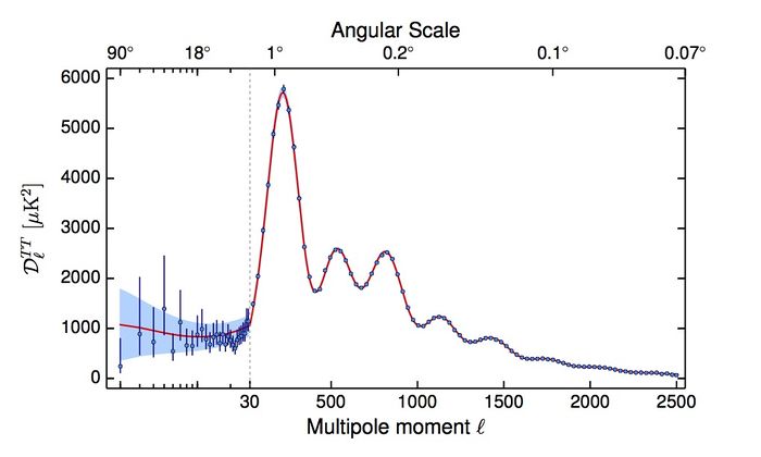
| − | The Planck best-fit CMB temperature power spectrum, shown in figure below, covers the wide range of multipoles <math> \ell </math> = 2-2508. Over the multipole range <math> \ell </math> = 2–29, the power spectrum is derived from a component-separation algorithm, ''Commander'', <span style="color:red"> UPDATE COMMANDER: applied to maps in the frequency range 30–353 GHz over 91% of the sky {{PlanckPapers|planck2013-p06}} . The asymmetric error bars associated to this spectrum are the 68% confidence limits and include the uncertainties due to foreground subtraction </span>. For multipoles greater than <math>\ell= | + | The Planck best-fit CMB temperature power spectrum, shown in figure below, covers the wide range of multipoles <math> \ell </math> = 2-2508. Over the multipole range <math> \ell </math> = 2–29, the power spectrum is derived from a component-separation algorithm, ''Commander'', <span style="color:red"> UPDATE COMMANDER: applied to maps in the frequency range 30–353 GHz over 91% of the sky {{PlanckPapers|planck2013-p06}} . The asymmetric error bars associated to this spectrum are the 68% confidence limits and include the uncertainties due to foreground subtraction </span>. For multipoles equal or greater than <math>\ell=30</math>, instead, the spectrum is derived from the ''Plik'' likelihood {{PlanckPapers|planck2014-a13}} by optimally combining the spectra in the frequency range 100-217 GHz, and correcting them for unresolved foregrounds. Associated 1-sigma errors include beam uncertainties. Both ''Commander'' and ''Plik'' are described in more details in the sections below. |
[[File: Planck2014 TT Dl NORES bin30 w180mm.jpeg|thumb|center|700px|'''CMB spectrum. Logarithmic x-scale up to <math>\ell=30</math>, linear at higher <math>\ell</math>; all points with error bars. The red line is the Planck best-fit primordial power spectrum (cf Planck TT+lowP in Table 3 of {{PlanckPapers|planck2014-a15}}).''']] | [[File: Planck2014 TT Dl NORES bin30 w180mm.jpeg|thumb|center|700px|'''CMB spectrum. Logarithmic x-scale up to <math>\ell=30</math>, linear at higher <math>\ell</math>; all points with error bars. The red line is the Planck best-fit primordial power spectrum (cf Planck TT+lowP in Table 3 of {{PlanckPapers|planck2014-a15}}).''']] | ||
| Line 14: | Line 14: | ||
The <math>\ell</math> < 50 part of the Planck power spectrum is derived from the Commander approach, which implements Bayesian component separation in pixel space, fitting a parametric model to the data by sampling the posterior distribution for the model parameters {{PlanckPapers|planck2013-p06}}. The power spectrum at any multipole <math>\ell</math> is given as the maximum probability point for the posterior <math>C_\ell</math> distribution, marginalized over the other multipoles, and the error bars are 68% confidence level {{PlanckPapers|planck2013-p08}}. | The <math>\ell</math> < 50 part of the Planck power spectrum is derived from the Commander approach, which implements Bayesian component separation in pixel space, fitting a parametric model to the data by sampling the posterior distribution for the model parameters {{PlanckPapers|planck2013-p06}}. The power spectrum at any multipole <math>\ell</math> is given as the maximum probability point for the posterior <math>C_\ell</math> distribution, marginalized over the other multipoles, and the error bars are 68% confidence level {{PlanckPapers|planck2013-p08}}. | ||
</span> | </span> | ||
| − | The <math>\ell</math> > 30 part of the CMB temperature power spectrum has been derived by the Plik likelihood, a code that implements a pseudo-Cl based technique, extensively described in Sec. 2 and the Appendix of {{PlanckPapers|planck2013-p08}}. Frequency spectra are computed as | + | The <math>\ell</math> > 30 part of the CMB temperature power spectrum has been derived by the Plik likelihood, a code that implements a pseudo-Cl based technique, extensively described in Sec. 2 and the Appendix of {{PlanckPapers|planck2013-p08}}. Frequency spectra are computed as cross-spectra between half-mission maps. Mask and multipole range choices for each frequency spectrum are summarized in Section 3.3 of {{PlanckPapers|planck2014-p15}} and in {{PlanckPapers|planck2014-p13}}. The final power spectrum is an optimal combination of the 100, 143, 143x217 and 217 GHz spectra, corrected for the best-fit unresolved foregrounds and inter-frequency calibration factors, as derived from the full likelihood analysis (cf Planck+TT+lowP in Table 3 of {{PlanckPapers|planck2014-p15}}). A thorough description of the models of unresolved foregrounds is given in {{PlanckPapers|planck2014-p13}}. The spectrum covariance matrix accounts for cosmic variance and noise contributions, together with beam uncertainties. Both spectrum and associated covariance matrix are available in two formats: |
| + | #Unbinned, in 2479 bandpowers. | ||
| + | #Binned, in 83 bandpowers. We bin the Cl power spectra with a weight proportional to <math> \ell (\ell+1) <\math> so that: | ||
| + | <math> | ||
| + | C_b=\Sigma_{\ell \in b} w_\ell C_\ell | ||
| + | w_\ell=\frac{\ell (\ell+1)}{\Sigma_\ell \in bin \ell (\ell+1)} | ||
| + | <\math> | ||
| + | |||
===Inputs=== | ===Inputs=== | ||
Revision as of 19:27, 3 February 2015
Contents
CMB spectra[edit]
General description[edit]
The Planck best-fit CMB temperature power spectrum, shown in figure below, covers the wide range of multipoles = 2-2508. Over the multipole range = 2–29, the power spectrum is derived from a component-separation algorithm, Commander, UPDATE COMMANDER: applied to maps in the frequency range 30–353 GHz over 91% of the sky Planck-2013-XII[1] . The asymmetric error bars associated to this spectrum are the 68% confidence limits and include the uncertainties due to foreground subtraction . For multipoles equal or greater than , instead, the spectrum is derived from the Plik likelihood Planck-2015-A11[2] by optimally combining the spectra in the frequency range 100-217 GHz, and correcting them for unresolved foregrounds. Associated 1-sigma errors include beam uncertainties. Both Commander and Plik are described in more details in the sections below.

Production process[edit]
UPDATE COMMANDER The < 50 part of the Planck power spectrum is derived from the Commander approach, which implements Bayesian component separation in pixel space, fitting a parametric model to the data by sampling the posterior distribution for the model parameters Planck-2013-XII[1]. The power spectrum at any multipole is given as the maximum probability point for the posterior distribution, marginalized over the other multipoles, and the error bars are 68% confidence level Planck-2013-XV[4]. The > 30 part of the CMB temperature power spectrum has been derived by the Plik likelihood, a code that implements a pseudo-Cl based technique, extensively described in Sec. 2 and the Appendix of Planck-2013-XV[4]. Frequency spectra are computed as cross-spectra between half-mission maps. Mask and multipole range choices for each frequency spectrum are summarized in Section 3.3 of [5] and in [6]. The final power spectrum is an optimal combination of the 100, 143, 143x217 and 217 GHz spectra, corrected for the best-fit unresolved foregrounds and inter-frequency calibration factors, as derived from the full likelihood analysis (cf Planck+TT+lowP in Table 3 of [5]). A thorough description of the models of unresolved foregrounds is given in [6]. The spectrum covariance matrix accounts for cosmic variance and noise contributions, together with beam uncertainties. Both spectrum and associated covariance matrix are available in two formats:
- Unbinned, in 2479 bandpowers.
- Binned, in 83 bandpowers. We bin the Cl power spectra with a weight proportional to ):
- frequency maps from 30–353 GHz
- common mask Planck-2013-XII[1]
- compact sources catalog
- High-l spectrum ()
- 100, 143, 143x217 and 217 GHz spectra and their covariance matrix (Sec. 2 in Planck-2013-XV[4])
- best-fit foreground templates and inter-frequency calibration factors (Table 5 of Planck-2013-XVI[7])
- Beam transfer function uncertainties Planck-2013-VII[8]
File names and Meta data[edit]
The CMB spectrum and its covariance matrix are distributed in a single FITS file named
which contains 3 extensions
- LOW-ELL (BINTABLE)
- with the low ell part of the spectrum, not binned, and for l=2-49. The table columns are
- ELL (integer): multipole number
- D_ELL (float): $D_l$ as described below
- ERRUP (float): the upward uncertainty
- ERRDOWN (float): the downward uncertainty
- HIGH-ELL (BINTABLE)
- with the high-ell part of the spectrum, binned into 74 bins covering in bins of width (with the exception of the last 4 bins that are wider). The table columns are as follows:
- ELL (integer): mean multipole number of bin
- L_MIN (integer): lowest multipole of bin
- L_MAX (integer): highest multipole of bin
- D_ELL (float): $D_l$ as described below
- ERR (float): the uncertainty
- COV-MAT (IMAGE)
- with the covariance matrix of the high-ell part of the spectrum in a 74x74 pixel image, i.e., covering the same bins as the HIGH-ELL table.
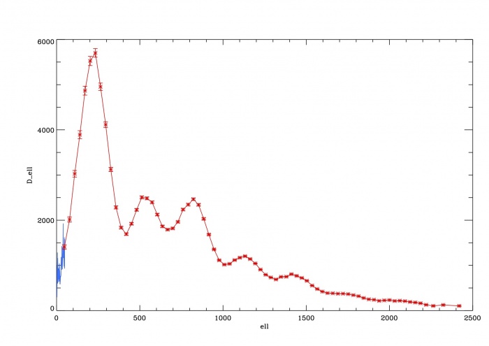
The spectra give $D_\ell = \ell(\ell+1)C_\ell / 2\pi$ in units of $\mu\, K^2$, and the covariance matrix is in units of $\mu\, K^4$. The spectra are shown in the figure below, in blue and red for the low- and high- parts, respectively, and with the error bars for the high-ell part only in order to avoid confusion.
The CMB spectrum is also given in a simple text comma-separated file:
Likelihood[edit]
TO BE WRITTEN.
References[edit]
- ↑ 1.01.11.2 Planck 2013 results. XI. Component separation, Planck Collaboration, 2014, A&A, 571, A11
- ↑ Planck 2015 results. XI. CMB power spectra, likelihoods, and robustness of cosmological parameters, Planck Collaboration, 2016, A&A, 594, A11.
- ↑ Planck 2015 results. XIII. Cosmological parameters, Planck Collaboration, 2016, A&A, 594, A13.
- ↑ 4.04.14.2 Planck 2013 results. XV. CMB power spectra and likelihood, Planck Collaboration, 2014, A&A, 571, A15
- ↑ 5.05.1
- ↑ 6.06.1
- ↑ Planck 2013 results. XVI. Cosmological parameters, Planck Collaboration, 2014, A&A, 571, A16
- ↑ Planck 2013 results. VII. HFI time response and beams, Planck Collaboration, 2014, A&A, 571, A7
Cosmic Microwave background
Flexible Image Transfer Specification
