Difference between revisions of "Map-making LFI"
(→Low-resolution maps and noise covariance matrices) |
|||
| (104 intermediate revisions by 8 users not shown) | |||
| Line 1: | Line 1: | ||
| − | == | + | ==Mapmaking== |
| − | + | The inputs to the mapmaking procedure consist of the calibrated timelines, along with the corresponding pointing information. | |
| − | The | ||
The main output consists of temperature and polarization maps. | The main output consists of temperature and polarization maps. | ||
| − | An important part of the | + | An important part of the mapmaking step is the removal of correlated 1/<i>f</i> noise. |
| − | LFI maps were constructed with the | + | LFI maps were constructed with the MADAM mapmaking code, version 3.7.4. |
| − | The code is based on generalized destriping technique, where the correlated noise component is | + | The code is based on a generalized destriping technique, where the correlated noise component is modelled as a sequence of constant offset "baselines". |
The baseline solution is constrained by a noise filter. | The baseline solution is constrained by a noise filter. | ||
| − | As auxiliary information the code produces a hit count map and a white noise covariance matrix. | + | As auxiliary information, the code produces a hit-count map and a white noise covariance matrix. |
| − | No beam information is used, | + | No beam information is used, with the signal being simply assigned to the pixel where the centre of the beam falls. |
| − | + | The chosen baseline length was 1s for the 44GHz and 70GHz maps, 0.25s for the 30GHz map. This gives good noise removal, | |
| − | without being computationally | + | without being computationally burdensome. |
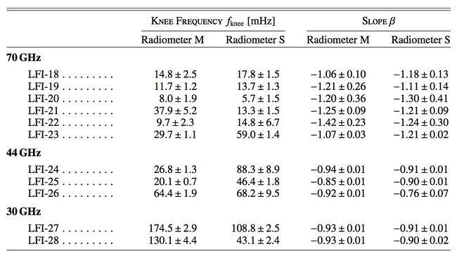
| − | The noise filter was built according to the noise parameters listed in Table | + | The noise filter was built according to the noise parameters listed in Table 1. |
| − | Flagged samples were excluded from the analysis. The | + | Flagged samples were excluded from the analysis. The Galaxy region was masked out in the destriping phase, to reduce errors arising from strong signal gradients. Radiometers were combined according to the horn-uniform weighting scheme to minimize systematics. The polarization component was included in the analysis, although only the temperature maps were released in 2013. |
| − | A detailed description of the | + | A detailed description of the mapmaking procedure is given in {{PlanckPapers|planck2013-p02}} {{PlanckPapers|planck2014-a03}} {{PlanckPapers|planck2014-a07}}. See also the section on [[Frequency Maps]]. |
| − | The maps are in | + | The maps are in HEALPix format, at resolution <i>N</i><sub>side</sub>=1024 for all frequencies with an additional map at <i>N</i><sub>side</sub>=2048 for the LFI 70GHz channel, in the nested pixelization scheme. |
Unobserved pixels are marked by a special value. | Unobserved pixels are marked by a special value. | ||
| − | The released maps are in | + | The released maps are in Galactic coordinates. |
| − | The conversion | + | The conversion between ecliptic and Galactic coordinates is described by the rotation matrix |
| − | + | <math> | |
| − | + | \newcommand{\Re}{\mathrm{Re}\,} | |
| − | + | \newcommand{\pFq}[5]{{}_{#1}\mathrm{F}_{#2} \left( \genfrac{}{}{0pt}{}{#3}{#4} \bigg| {#5} \right)} | |
| + | </math> | ||
| + | |||
| + | :<math> | ||
| + | \begin{align} | ||
| + | \label{def:Rot_matrix} | ||
| + | \left (\begin{matrix} | ||
| + | -0.054882486 & 0.494116468 & -0.867661702\\ | ||
| + | -0.993821033 & -0.110993846 & -0.000346354\\ | ||
| + | -0.096476249 & 0.86228144 & 0.497154957 | ||
| + | \end{matrix} \right). | ||
| + | \end{align} | ||
| + | </math> | ||
The conversion was applied to the input pointing data, prior to the construction of the map. | The conversion was applied to the input pointing data, prior to the construction of the map. | ||
| + | [[File:lfi_noise.jpg|650px]] | ||
| + | :<small>'''Table 1: Knee frequencies and slopes for the LFI radiometers.'''</small> | ||
| + | <!-- | ||
| + | {| class="wikitable" align="center" style="text-align:center" border="1" cellpadding="5" cellspacing="0" | ||
| + | |+ '''Table 1: Noise parameters used in the construction of the noise filter, and the radiometer weights.''' | ||
| + | |-bgcolor="ffdead" | ||
| + | !Radiometer || White noise sigma [mK<math>_{\rm CMB}</math>] || Slope ||Knee frequency [mHz] || <math>f_{\rm min}</math> [Hz] || Horn-uniform weight | ||
| + | |- | ||
| + | |'''LFI18M''' || 4.542 || -1.07 || 15.3 || 1.15e-5 || 5.297E+04 | ||
| + | |- | ||
| + | |'''LFI18S''' || 4.139 || -1.20 || 18.3 || 1.15e-5 || 5.297E+04 | ||
| + | |- | ||
| + | |'''LFI19M''' || 5.146 || -1.22 || 11.9 || 1.15e-5 || 3.948E+04 | ||
| + | |- | ||
| + | |'''LFI19S''' || 4.918 || -1.12 || 14.6 || 1.15e-5 || 3.948E+04 | ||
| + | |- | ||
| + | |'''LFI20M''' || 5.214 || -1.31 || 8.4 || 1.15e-5 || 3.482E+04 | ||
| + | |- | ||
| + | |'''LFI20S''' || 5.500 || -1.34 || 6.0 || 1.15e-5 || 3.482E+04 | ||
| + | |- | ||
| + | |'''LFI21M''' || 4.008 || -1.26 || 39.3 || 1.15e-5 || 4.897E+04 | ||
| + | |- | ||
| + | |'''LFI21S''' || 4.978 || -1.24 || 14.0 || 1.15e-5 || 4.897E+04 | ||
| + | |- | ||
| + | |'''LFI22M''' || 4.348 || -1.53 || 10.1 || 1.15e-5 || 4.864E+04 | ||
| + | |- | ||
| + | |'''LFI22S''' || 4.713 || -1.20 || 15.9 || 1.15e-5 || 4.864E+04 | ||
| + | |- | ||
| + | |'''LFI23M''' || 4.468 || -1.07 || 30.2 || 1.15e-5 || 4.670E+04 | ||
| + | |- | ||
| + | |'''LFI23S''' || 4.782 || -1.21 || 58.8 || 1.15e-5 || 4.670E+04 | ||
| + | |- | ||
| + | |'''LFI24M''' || 3.145 || -0.94 || 26.9 || 1.15e-5 || 1.158E+05 | ||
| + | |- | ||
| + | |'''LFI24S''' || 2.717 || -0.91 || 73.0 || 1.15e-5 || 1.158E+05 | ||
| + | |- | ||
| + | |'''LFI25M''' || 2.821 || -0.85 || 20.1 || 1.15e-5 || 1.319E+05 | ||
| + | |- | ||
| + | |'''LFI25S''' || 2.684 || -0.90 || 46.1 || 1.15e-5 || 1.319E+05 | ||
| + | |- | ||
| + | |'''LFI26M''' || 3.280 || -0.92 || 64.4 || 1.15e-5 || 1.056E+05 | ||
| + | |- | ||
| + | |'''LFI26S''' || 2.859 || -0.88 || 43.8 || 1.15e-5 || 1.056E+05 | ||
| + | |- | ||
| + | |'''LFI27M''' || 1.609 || -0.93 || 175.1 || 1.15e-5 || 3.567E+05 | ||
| + | |- | ||
| + | |'''LFI27S''' || 1.737 || -0.91 || 109.6 || 1.15e-5 || 3.567E+05 | ||
| + | |- | ||
| + | |'''LFI28M''' || 1.814 || -0.93 || 127.9 || 1.15e-5 || 3.353E+05 | ||
| + | |- | ||
| + | |'''LFI28S''' || 1.635 || -0.91 || 43.9 || 1.15e-5 || 3.353E+05 | ||
| + | |} | ||
| + | --> | ||
| − | + | ==Low-resolution maps and noise covariance matrices== | |
| − | + | To fully exploit the information contained in the large-scale structure of the microwave sky, pixel-pixel covariances are needed in the maximum likelihood estimation of the CMB power spectrum. However, full covariance matrices are impossible to employ at the native map resolution due to resource limitations. A low-resolution data set is therefore required for the low-ℓ analysis. This data set has been packed into three different files, one per frequency, called "LFI_NoiseCovMat_0??_0016_R2.00.tgz", that can be downloaded from the Cosmology section of the Planck Legacy Archive. | |
| − | + | They consist of low-resolution maps, and descriptions of residual noise present in those maps given by pixel-pixel noise covariance matrices (NCVMs). | |
| − | |||
| − | - | ||
| − | |||
| − | - | ||
| − | |||
| − | - | ||
| − | |||
| − | - | ||
| − | |||
| − | - | ||
| − | + | {| border="1" cellpadding="3" cellspacing="0" align="center" style="text-align:left" width=800px | |
| + | |+ Contents of '''LFI_NoiseCovMat_0??_0016_R2.00.tgz''' | ||
| + | |- bgcolor="ffdead" | ||
| + | ! Filenames || Comment | ||
| + | |- | ||
| + | | LFI_SkyMap_0??_0016_nobs_DX11D_full_regnoise.fits || Low-resolution maps. Full mission coverage. | ||
| + | |- | ||
| + | | LFI_SkyMap_0??_0016_nobs_DX11D_s1-s3-s5-s6-s7-s8_regnoise.fits || Low-resolution maps. Full mission coverage, excluding Surveys 2 and 4. | ||
| + | |- | ||
| + | | offset_covmat_toast_nside64T16_nobs_025sec_??GHz_DX11D_full_bin.dat || Low-resolution noise covariance matrices. Regularization noise added. Format: C unformatted. | ||
| + | |- | ||
| + | | offset_covmat_toast_nside64T16_nobs_025sec_??GHz_DX11D_s1-s3-s5-s6-s7-s8_bin.dat || Low-resolution noise covariance matrices. Regularization noise added. Format: C unformatted. | ||
| + | |- | ||
| + | | covmat_toast_nside64T16_nobs_025sec_??GHz_DX11D_full_bin.dat || Low-resolution noise covariance matrices. No regularization noise added. Format: C unformatted. | ||
| + | |- | ||
| + | | covmat_toast_nside64T16_nobs_025sec_??GHz_DX11D_s1-s3-s5-s6-s7-s8_bin.dat || Low-resolution noise covariance matrices. No regularization noise added. Format: C unformatted. | ||
| + | |- | ||
| + | | DX11D_0??_016_full_conv060_VarianceBPcorrection_v2.fits || Variance of the BandPass correction. | ||
| + | |- | ||
| + | | DX11D_0??_016_full_conv060_BPcorrection_v2.fits || BandPass Correction map to be SUBTRACTED to the corresponding Low Resolution. | ||
| + | |- | ||
| + | | QUmask_DX11_16_0??GHz_R1.50.fits || | ||
| + | |- | ||
| + | |} | ||
| − | |||
| − | |||
| − | |||
| − | |||
| − | |||
| − | |||
| − | |||
| − | |||
| − | |||
| − | |||
| + | The low-resolution data set can currently be utilized efficiently only at resolution <i>N</i><sub>side</sub> = 16, or lower. All the low-resolution data products are produced at this target resolution. | ||
| + | ===Low-resolution maps=== | ||
| + | A number of different schemes to obtain the low-resolution maps are discussed in {{BibCite|keskitalo2013}}. We chose to downgrade the maps using the inverse noise weighting. This is discussed further in {{PlanckPapers|planck2013-p02}} {{PlanckPapers|planck2014-a07}}. | ||
====Inputs==== | ====Inputs==== | ||
| − | + | We took the high-resolution maps described in [[Map-making LFI#Map-making|Map-making]] and [[Frequency Maps]], and the corresponding 3×3 matrices as an input for this analysis step. | |
| − | We took the high resolution maps described in LFI-Map-making and the corresponding | ||
====Production==== | ====Production==== | ||
| + | The high-resolution maps were downgraded to <i>N</i><sub>side</sub> = 16 using inverse noise weights (given by the 3×3 matrices), and subsequently the temperature part was smoothed with a symmetric Gaussian beam with FWHM = 440arcmin. | ||
| − | + | ===Noise covariance matrices=== | |
| − | |||
| − | ===Noise | ||
| − | The statistical description of the residual noise in the maps is given in the form of a pixel-to-pixel noise covariance matrix (NCVM), as described in | + | The statistical description of the residual noise in the maps is given in the form of a pixel-to-pixel noise covariance matrix (NCVM), as described in {{BibCite|keskitalo2013}}. |
====Inputs==== | ====Inputs==== | ||
| − | The noise model was | + | The noise model was determined by three noise parameters: the white noise level σ; slope; and knee frequency <i>f</i><sub>knee</sub>. We actually used three sets of noise parameters, one for the entire mission (noise parameters are listed in Table 1), and one for each sky survey (SS1 and SS2). |
| − | We used the same pointing as in the noise Monte Carlo simulations. See the description in Noise Monte Carlo | + | We used the same pointing as in the noise Monte Carlo simulations. See the description in [[Map-making LFI#Noise Monte Carlo Simulation#Inputs|Noise Monte Carlo Simulation Inputs]]. |
| − | We used the gap files produced during the making of the flight maps to leave out samples that were flagged bad for various reasons. | + | We used the gap files produced during the making of the flight maps to leave out samples that were flagged as bad for various reasons. |
====Production==== | ====Production==== | ||
| − | The output of the NCVM module of | + | The output of the NCVM module of MADAM mapmaker are inverse NCVMs. Since the inverse matrices are additive, we divided the computations into a number of small chunks to save computational resources. We first calculated one inverse NCVM per radiometer per survey at resolution <i>N</i><sub>side</sub>=32, and then combined these individual inverse matrices to form the actual inverse matrices. The mapmaking parameters were almost identical to the standard mapmaking runs. The differing parameter values are listed below: |
| − | + | * baseline lengths were 0.25s (eight samples), 0.50s (24 samples), and 0.50s (39 samples) for 30GHz, 44GHz, and 70GHz, respectively; | |
| − | + | * the calculations were performed at resolution <i>N</i><sub>side</sub> = 32; | |
| − | + | * no destriping mask was applied; | |
| − | + | * the horns were weighted optimally. | |
| − | |||
| − | - | + | To obtain the noise covariance from its inverse, the matrices are inverted using the eigen decomposition of a matrix. The monopole of the temperature map cannot be resolved by the mapmaker, and thus the matrix becomes singular. This ill-determined mode is left out of the analysis. |
| − | + | Having calculated the eigen decomposition in the previous step, we can apply the same linear operators to modify the eigenvectors as were applied to the high-resolution maps while downgrading them. The eigenvectors are downgraded to <i>N</i><sub>side</sub> = 16 using inverse noise weights, and subsequently the temperature part is smoothed with a symmetric Gaussian beam with FWHM = 440arcmin. | |
| − | |||
| − | |||
| − | Having calculated the eigen decomposition in the previous step, we can apply the same linear operators to modify the eigenvectors as | ||
The final matrices are then recomposed from the original eigenvalues and modified eigenvectors. | The final matrices are then recomposed from the original eigenvalues and modified eigenvectors. | ||
| − | The low resolution noise covariance matrices | + | The low-resolution noise covariance matrices: |
| − | + | * are C binary format files; | |
| − | + | * are organized in block form, | |
| − | + | <math> | |
| − | + | \newcommand{\Re}{\mathrm{Re}\,} | |
| − | + | \newcommand{\pFq}[5]{{}_{#1}\mathrm{F}_{#2} \left( \genfrac{}{}{0pt}{}{#3}{#4} \bigg| {#5} \right)} | |
| + | </math> | ||
| + | <math> | ||
| + | \begin{align} | ||
| + | \label{def:Block_form} | ||
\left (\begin{matrix} | \left (\begin{matrix} | ||
II & IQ & IU \\ | II & IQ & IU \\ | ||
QI & QQ & QU \\ | QI & QQ & QU \\ | ||
UI & UQ & UU | UI & UQ & UU | ||
| − | \end{matrix} \right) | + | \end{matrix} \right); |
| − | + | \end{align} | |
| − | + | </math> | |
| + | |||
| + | * are in the HEALPix nested pixelisation scheme (with resolution is <i>N</i><sub>side</sub> = 16, and thus there are <i>N</i><sub>pix</sub> = 3072 pixels); | ||
| + | * are in Galactic coordinates; | ||
| + | * have K<sub>CMB</sub> units. | ||
| + | |||
| + | ==Half-ring jackknife noise maps== | ||
| − | + | ===Overview=== | |
| − | - | + | In order to estimate the noise directly at the map level and in the angular power spectra, we divided the time-ordered data into two halves and produced half-ring jackknife maps, as described in {{PlanckPapers|planck2014-a03||Planck-2015-A03}}. |
| − | - | + | Briefly, instead of using the full time-ordered data as described above, we produced two sets of maps using either only the first half of each pointing period (map named <b>j</b><sub>1</sub> below) or only the second half of each pointing period (map named <b>j</b><sub>2</sub>). At each pixel <i>p</i>, these half-ring jackknife maps <b>j</b><sub>1</sub> and <b>j</b><sub>2</sub> contain the same sky signal, since they result from the same scanning pattern on the sky. However, because of instrumental noise, the maps <b>j</b><sub>1</sub> and <b>j</b><sub>2</sub> are not identical. |
| − | - | + | We estimated the noise level in each map <b>m</b> made using the full (ring) data, by constructing a half-ring difference map |
| − | - | + | <math>\mathbf{n_{m}}(p) = [ \mathbf{j_1}(p) - \mathbf{j_2}(p)] \ / \ \mathbf{w_{\rm hit}}(p)\,,</math> |
| − | + | with weights | |
| − | = | + | <math>\mathbf{w_{hit}}(p) = \sqrt{ \mathbf{hit_{full}}(p) \left[ \frac{1}{\mathbf{hit_1}(p)} + |
| + | \frac{1}{\mathbf{hit_2}(p)} \right]}\,</math>. | ||
| − | == | + | Here <b>hit</b><sub>full</sub>(<i>p</i>) = <b>hit</b><sub>1</sub>(<i>p</i>) + <b>hit</b><sub>2</sub>(<i>p</i>) |
| + | is the hit count at pixel <i>p</i> in the full map <b>m</b>, while <b>hit</b><sub>1</sub> and <b>hit</b><sub>2</sub> are the hit counts of <b>j</b><sub>1</sub> and <b>j</b><sub>2</sub>, respectively. The weight factor <b>w</b><sub>hit</sub>(<i>p</i>) is equal to 2 only in those pixels where <b>hit</b><sub>1</sub>(<i>p</i>) = <b>hit</b><sub>2</sub>(<i>p</i>) . In a typical pixel, <b>hit</b><sub>1</sub>(<i>p</i>) will differ slightly from | ||
| + | <b>hit</b><sub>2</sub>(<i>p</i>) and hence the weight factor is <b>w</b><sub>hit</sub>(<i>p</i>)>2. | ||
| − | + | The half-ring difference maps <b>n</b><sub>m</sub> are the most direct measure of the noise in the actual maps. The other noise estimates (NCVM and noise Monte Carlo) rely on specific modelling of the noise and this modelling can be validated by comparing to the half-ring difference maps. However, the half-ring difference maps can only capture the noise that varies faster than half of the duration of the pointing period, i.e., the noise whose frequency is approximately <i>f</i> > 1/20min = 0.85mHz. | |
| − | + | We calculated the noise maps <b>n</b><sub>m</sub>, from half-ring "jackknife" maps for temperature (<i>I</i>) and polarization (<i>Q</i> and <i>U</i>) and as a first quality check of the maps (and as one of the tests of the whole data processing pipeline up to the map level) tested both numerically and visually that these noise maps divided pixel-by-pixel by the square root of the white noise covariance maps were approximately Gaussian with variance near to unity. Temperature noise maps for the nominal survey and for the first and second sky surveys are shown in the next subsection. Furthermore we calculated from the noise maps the temperature and polarization (E and B mode) auto-correlation and cross-correlation noise angular power spectra using HEALPix anafast and compared to these the results from the white noise covariance matrices and from the noise Monte Carlo simulations. A similar comparison was made between downgraded half-ring noise maps, downgraded noise Monte Carlo maps, and the low-resolution noise covariance maps. Detailed results are presented in {{PlanckPapers|planck2014-a04}}. | |
| − | + | ===Examples of half-ring difference maps and noise angular power spectra=== | |
| − | + | ====Hit-count weighted half-ring difference maps==== | |
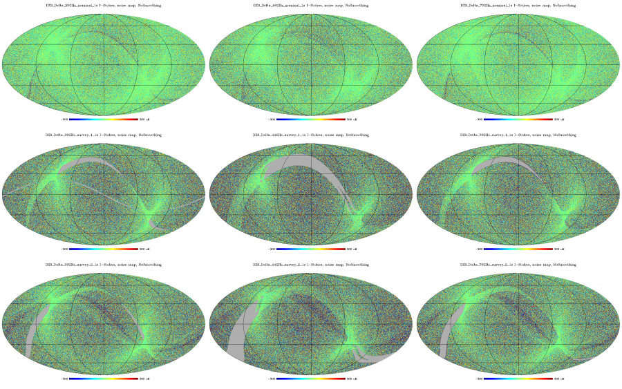
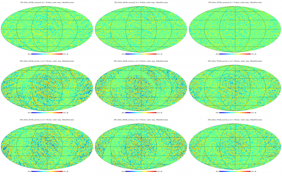
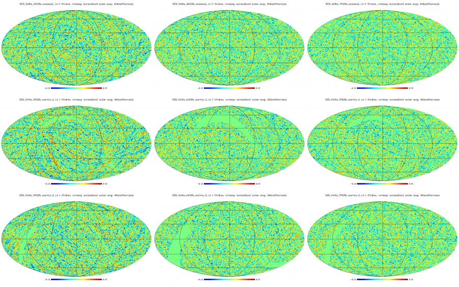
| − | + | Here we show some hit-count weighted half-ring difference maps, i.e., noise maps for temperature. The columns are for different LFI frequencies, namely 30GHz, 44GHz, and 70GHz. The rows are for the nominal survey (a bit more than 1 year of observations), Survey 1 (the first sky survey, approximately the first half year of observations) and Survey 2 (the second sky survey, approximately the second half year of observations). Some features are visible, particularly in the Galactic plane; these are due to "gradient leakage." In regions where the gradient in the sky signal is very large, even a tiny difference in the pointing of the first and second half of each pointing period causes the signal to "leak" into the half-ring difference map. In practice this is not a problem for noise estimation, since these regions (i.e., the Galaxy, Orion, Crab Nebula, etc.) will be masked in the cosmology analysis. | |
| − | + | [[File:LFI_4_5_5_3_DX9_Delta_TemperatureNoiseMap_1s_frequency_and_SScomparison_NoSmoothing.png|thumb|900px|center|<b>Half-ring difference maps. These are calculated at the native <i>N</i><sub>side</sub>=1024 resolution (note for the LFI 70GHz channel maps are also generated at <i>N</i><sub>side</sub>=2048). The columns are frequency (30, 44, and 70GHz), while the rows are sky surveys (Nominal, Survey 1, and Survey 2).</b>]] | |
| − | |||
| − | + | [[File:LFI_4_5_5_3_DX9_Delta_TemperatureNoiseMap_1s_frequency_and_SScomparison_fwhm60arcmin.png|thumb|900px|center|<b>Half-ring difference maps (the same as above, but) <i>smoothed</i> with a 60 arcmin FWHM Gaussian. The columns are frequency (30, 44, and 70GHz), while the rows are sky surveys (Nominal, Survey 1, and Survey 2).</b>]] | |
| − | |||
| − | |||
| − | + | ====Normalized hit-count weighted half-ring difference maps==== | |
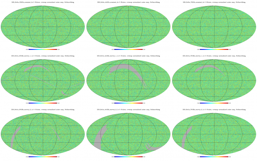
| − | + | Now we show the same as above, but divided by the square root of the estimate of the white noise variance in each pixel. These normalized noise maps should be approximately Gaussian with unit variance (at the native resolution), apart from some stripes that are due to correlated (non-Gaussian) 1/<i>f</i> noise. The large-scale 1/<i>f</i> noise is more apparent in the smoothed version of the figure, which follows after the native resolution version. | |
| − | |||
| − | + | [[File:LFI_4_5_5_3_DX9_Delta_NormalizedTemperatureNoiseMap_1s_frequency_and_SScomparison_NoSmoothing.png|thumb|900px|center|<b>Normalized half-ring difference maps calculated at the native <i>N</i><sub>side</sub>=1024 resolution (note for the LFI 70GHz channel maps are also generated at <i>N</i><sub>side</sub>=2048). Columns are frequency (30, 44, and 70GHz), while rows are sky surveys (Nominal, Survey 1, and Survey 2).</b>]] | |
| − | |||
| − | < | + | [[File:LFI_4_5_5_3_DX9_Delta_NormalizedTemperatureNoiseMap_1s_frequency_and_SScomparison_fwhm60arcmin.png|thumb|900px|center|<b>Normalized half-ring difference maps (the same as above, but) smoothed with a 60 arcmin FWHM Gaussian. Columns are frequency (30, 44, and 70GHz), while rows are sky surveys (Nominal, Survey 1, and Survey 2).</b>]] |
| − | |||
| − | + | ====Noise angular power spectra from half-ring difference maps==== | |
| − | |||
| − | + | The noise angular power spectra are shown below. These were calculated using HEALPix routine anafast from half-ring difference temperature maps and normalized by the sky coverage to estimate the noise level if there was a full sky coverage. This enables us more easily to compare different surveys. | |
| − | + | [[File:LFI_4_5_5_3_DX9_Delta_SSnoiseComparison_loglin_TT.png|thumb|900px|center|<b>Columns are frequency (30, 44, and 70GHz). The Nominal mission map is black, Survey 1 is red, and Survey 2 is blue.</b>]] | |
| − | + | ===Comparison of noise estimates=== | |
| − | |||
| − | + | Here we compare noise angular power spectra estimated from half-ring difference maps (red) to the estimate from white noise covariance maps (blue), and the full noise Monte Carlo simulations (BLACK, top curve 16th percentile, middle curve 50th percentile, i.e., median, and bottom curve 84th percentile). See the next section for the details of noise Monte Carlos. | |
| − | |||
| − | |||
| − | + | [[File:DX9_Delta_noise_comparison_nominal_nomask.png|thumb|900px|center|<b>Nominal Survey.</b>]] | |
| − | [[File: | ||
| − | + | [[File:DX9_Delta_noise_comparison_survey1_nomask.png|thumb|900px|center|<b>Survey 1.</b>]] | |
| − | + | [[File:DX9_Delta_noise_comparison_survey2_nomask.png|thumb|900px|center|<b>Survey 2.</b>]] | |
| − | + | ====High-ell average noise relative to white noise estimate==== | |
| − | |||
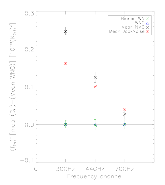
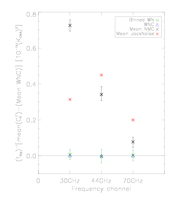
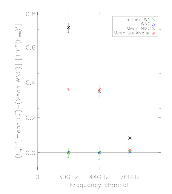
| − | + | The figure below is the same as the previous figures, but here the noise comparison is made from the high ℓ tails of the angular power spectra, where the white noise dominates. We have taken the average of <i>C</i><sub>ℓ</sub> from multipoles between 1150 and 1800, and subtracted the white noise estimate. The half-ring difference noise estimate is shown in red, the full noise Monte Carlo estimate in black, and the white noise estimate from noise Monte Carlos in green. The white noise estimate from the white noise covariance map (WNC), in blue, has been subtracted from all the results. | |
| − | |||
| − | |||
| − | |||
| − | + | [[File:Comparison_Cls_NMC_WNC_JN_WNCmean_removed_nominal_nomask.png|thumb|700px|center|<b>Nominal survey.</b>]] | |
| − | |||
| − | |||
| − | + | [[File:Comparison_Cls_NMC_WNC_JN_WNCmean_removed_survey1_nomask.png|thumb|700px|center|<b>Survey 1.</b>]] | |
| − | [[File:Comparison_Cls_NMC_WNC_JN_WNCmean_removed_survey1_nomask.png]] | ||
| − | |||
| − | |||
| + | [[File:Comparison_Cls_NMC_WNC_JN_WNCmean_removed_survey2_nomask.png|thumb|700px|center|<b>Survey 2.</b>]] | ||
| − | ==Noise Monte Carlo | + | ==Noise Monte Carlo simulations== |
===Overview=== | ===Overview=== | ||
Calculating and handling full pixel-to-pixel noise covariance matrices for Planck maps if feasible only at low resolution. | Calculating and handling full pixel-to-pixel noise covariance matrices for Planck maps if feasible only at low resolution. | ||
| − | To support the analysis of high-resolution maps, a Monte Carlo set of noise maps were produced. These maps were produced from noise timelines using the same map-making procedure as for the flight data. In the noise Monte Carlo it was possible to follow exactly the | + | To support the analysis of high-resolution maps, a Monte Carlo set of noise maps were produced. These maps were produced from noise timelines using the same map-making procedure as for the flight data. In the noise Monte Carlo it was possible to follow exactly the mapmaking procedure used for the flight maps, whereas for the calculation of noise covariance matrices some approximations had to be made. |
| − | Such noise Monte Carlos were produced at two levels of the analysis: 1) LFI Monte Carlo (MC) as part of the LFI data processing | + | Such noise Monte Carlos were produced at two levels of the analysis: (1) LFI Monte Carlo (MC) as part of the LFI data processing procedure; and (2) Full Focal Plane (FFP) Monte Carlos as part of the joint HFI/LFI data processing. This page describes the LFI noise MCs. For the FFP MC, see [[HL-sims]] and [[Simulation data]]. |
===Inputs=== | ===Inputs=== | ||
| − | The noise MC uses a three-parameter | + | The noise MC uses a three-parameter noise model, consisting of white noise level (σ), slope, and knee frequency (<i>f</i><sub>knee</sub>)). Here the noise consists of white noise and correlated 1/<i>f</i> noise, with a power spectrum |
| − | : | + | :<math> P(f) = \frac{2\sigma^2}{f_\mathrm{sample}}\left(\frac{f}{f_\mathrm{knee}}\right)^\mathrm{slope} </math>, |
| − | + | where <i>f</i><sub>sample</sub> is the sampling frequency of the instrument. The noise parameters were determined separately for each radiometer, as described in the section [[TOI processing LFI#Noise| Noise]] above, assuming they stayed constant over the mission. | |
| − | The detector pointing was reconstructed from satellite pointing, focal-plane geometry, pointing correction (tilt angle), and sample timing, using Level-S simulation software. The same pointing solution (two focal planes) was used as for the LFI flight maps. Due to numerical accuracy, the detector pointing in the noise MC was not exactly the same as for the flight maps, | + | The detector pointing was reconstructed from satellite pointing information, focal-plane geometry, pointing correction (tilt angle), and sample timing, using Level-S simulation software. The same pointing solution (two focal planes) was used as for the LFI flight maps. Due to numerical accuracy, the detector pointing in the noise MC was not exactly the same as for the flight maps, so some data samples (of the order of one in a thousand) whose pointing was near the pixel boundary ended up assigned to the neighbouring pixel. During mapmaking from the flight data, a "gap file" was produced to represent the samples that were omitted from mapmaking due to various flags. This gap file was used in the noise MC instead of the full set of flags. The flight mapmaking procedure used destriping masks to prevent regions of strong signal gradients from contributing to the noise baseline solution. These same destriping masks (one for each frequency channel) were used for the noise MC. |
===Production=== | ===Production=== | ||
| − | The noise was generated internally in the Madam | + | The noise was generated internally in the Madam mapmaking code using a stochastic differential equation (SDE) method, to avoid time-consuming writing and reading of noise timelines to and from disk. Noise for each pointing period was generated separately, using a double-precision random number seed constructed from the realization number, radiometer number, and the pointing period number; this allowed for regeneration of the same noise realization when needed. White noise and 1/<i>f</i> noise were generated separately. |
| − | The same | + | The same mapmaking code (Madam) with the same parameter settings was used for the noise MC as for the flight maps. |
| − | In addition to the destriped maps from the full noise (output maps), | + | In addition to the destriped maps from the full noise (output maps), binned maps from just the white noise (binned white noise maps) were produced; they represent the white noise part of the output maps. The difference between these two maps represents the residual correlated noise in the output map. The maps were made at HEALPix resolution <i>N</i><sub>side</sub> = 1024 for all LFI frequency channels and also at HEALPix resolution <i>N</i><sub>side</sub> = 2048 for the 70 GHz channel. |
| − | For low-resolution analysis, these maps were downgraded (and the temperature part was smoothed) to | + | For low-resolution analysis, these maps were downgraded (and the temperature part was smoothed) to <i>N</i><sub>side</sub> = 32 and <i>N</i><sub>side</sub> = 16. |
| − | + | In addition to frequency maps for the nominal survey, also single-survey and 70 GHz horn-pair maps were produced in the noise MC. For each case 102-1026 realizations were produced. | |
===Usage=== | ===Usage=== | ||
| − | These noise Monte Carlo maps were used for a number of | + | These noise Monte Carlo maps were used for a number of purposes in LFI data analysis. They were compared to the low-resolution noise covariance matrices, generated for the same noise model, in order to reveal the impact of the approximations in the noise covariance matrix calculation. They were compared to the half-ring noise maps to see how well the noise model matches the noise in the flight maps (noting, however, that the half-ring noise maps misrepresent the lowest noise frequencies in the flight maps, and contain some effects from the sky signal). They were also used in power spectrum estimation and non-Gaussianity estimation. |
===Examples=== | ===Examples=== | ||
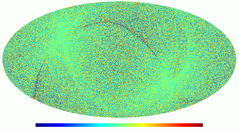
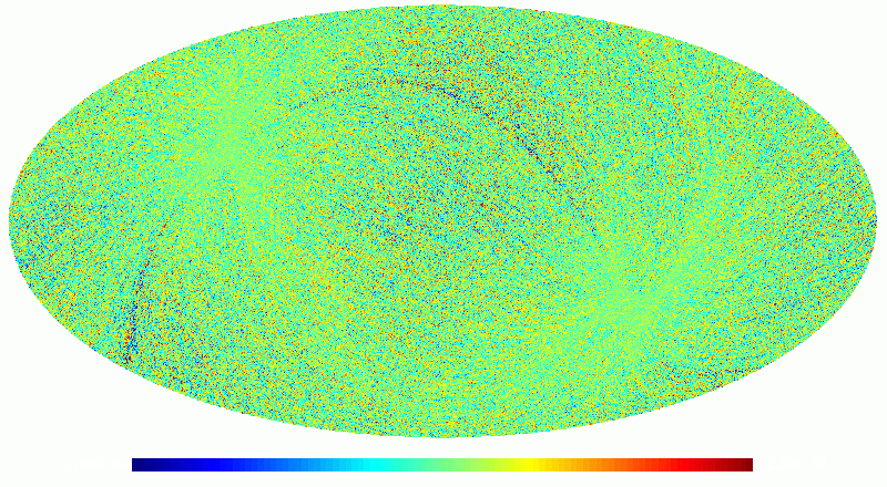
| − | As an example, we show below images of the first realization of the | + | As an example, we show below images of the first realization of the 70GHz frequency map noise for the nominal survey. The images are in the order: destriped full noise; binned white noise; and residual correlated noise. Note that it is difficult to see any difference between the first two images, since the residual correlated noise is more than an order of magnitude below the white noise level. The units here are K<sub>CMB</sub>. |
| + | |||
| + | |||
| + | |||
| + | [[File:LFI_4_5_5_4_madam_mask_1sec_DB10_1_noise_70GHz_all_DX9delta_nom_1024outmap.00000.gif|thumb|800px|center|<b>Destriped full noise.</b>]] | ||
| + | [[File:LFI_4_5_5_4_madam_mask_1sec_DB10_1_white_70GHz_all_DX9delta_nom_1024binmap.00000.gif|thumb|800px|center|<b>Binned white noise.</b>]] | ||
| + | [[File:LFI_4_5_5_4_madam_mask_1sec_DB10_1_rcnoise_70GHz_all_DX9delta_nom_1024map.00000.gif|thumb|800px|center|<b>Residual correlated noise.</b>]] | ||
| + | |||
| + | |||
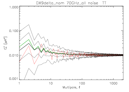
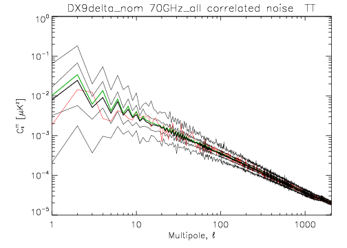
| + | The following two images show the statistics of the angular power spectra of 101 realizations of the 70 GHz frequency map noise for the nominal survey. The thick black line shows the median <i>C</i><sub>ℓ</sub>, while the green line the mean <i>C</i><sub>ℓ</sub>. Thin black lines show the minimum, 16th percentile, 84th percentile, and the maximum <i>C</i><sub>ℓ</sub>. The red line is the 102nd realization. The first plot is for the full noise in the output map, while the second plot is for the residual correlated noise. | ||
| + | |||
| + | [[File:LFI_4_5_5_4_cl_TT_stat_noisemc101_1sec_70GHz_all_DX9delta_nom.png|thumb|800px|center|<b>Full noise.</b>]] | ||
| + | [[File:LFI_4_5_5_4_cl_TT_stat_rcnoisemc101_1sec_70GHz_all_DX9delta_nom.png|thumb|800px|center|<b>Residual correlated noise.</b>]] | ||
| − | + | ==References== | |
| − | |||
| − | |||
| − | |||
| − | + | <References /> | |
| − | |||
| − | |||
| − | |||
| − | |||
| − | |||
| − | [[Category: | + | [[Category:LFI data processing|004]] |
Latest revision as of 15:33, 1 March 2017
Contents
Mapmaking[edit]
The inputs to the mapmaking procedure consist of the calibrated timelines, along with the corresponding pointing information. The main output consists of temperature and polarization maps. An important part of the mapmaking step is the removal of correlated 1/f noise.
LFI maps were constructed with the MADAM mapmaking code, version 3.7.4. The code is based on a generalized destriping technique, where the correlated noise component is modelled as a sequence of constant offset "baselines". The baseline solution is constrained by a noise filter. As auxiliary information, the code produces a hit-count map and a white noise covariance matrix. No beam information is used, with the signal being simply assigned to the pixel where the centre of the beam falls.
The chosen baseline length was 1s for the 44GHz and 70GHz maps, 0.25s for the 30GHz map. This gives good noise removal, without being computationally burdensome. The noise filter was built according to the noise parameters listed in Table 1.
Flagged samples were excluded from the analysis. The Galaxy region was masked out in the destriping phase, to reduce errors arising from strong signal gradients. Radiometers were combined according to the horn-uniform weighting scheme to minimize systematics. The polarization component was included in the analysis, although only the temperature maps were released in 2013. A detailed description of the mapmaking procedure is given in Planck-2013-II[1]Planck-2015-A02[2]Planck-2015-A06[3]. See also the section on Frequency Maps.
The maps are in HEALPix format, at resolution Nside=1024 for all frequencies with an additional map at Nside=2048 for the LFI 70GHz channel, in the nested pixelization scheme. Unobserved pixels are marked by a special value.
The released maps are in Galactic coordinates. The conversion between ecliptic and Galactic coordinates is described by the rotation matrix
The conversion was applied to the input pointing data, prior to the construction of the map.
- Table 1: Knee frequencies and slopes for the LFI radiometers.
Low-resolution maps and noise covariance matrices[edit]
To fully exploit the information contained in the large-scale structure of the microwave sky, pixel-pixel covariances are needed in the maximum likelihood estimation of the CMB power spectrum. However, full covariance matrices are impossible to employ at the native map resolution due to resource limitations. A low-resolution data set is therefore required for the low-ℓ analysis. This data set has been packed into three different files, one per frequency, called "LFI_NoiseCovMat_0??_0016_R2.00.tgz", that can be downloaded from the Cosmology section of the Planck Legacy Archive. They consist of low-resolution maps, and descriptions of residual noise present in those maps given by pixel-pixel noise covariance matrices (NCVMs).
| Filenames | Comment |
|---|---|
| LFI_SkyMap_0??_0016_nobs_DX11D_full_regnoise.fits | Low-resolution maps. Full mission coverage. |
| LFI_SkyMap_0??_0016_nobs_DX11D_s1-s3-s5-s6-s7-s8_regnoise.fits | Low-resolution maps. Full mission coverage, excluding Surveys 2 and 4. |
| offset_covmat_toast_nside64T16_nobs_025sec_??GHz_DX11D_full_bin.dat | Low-resolution noise covariance matrices. Regularization noise added. Format: C unformatted. |
| offset_covmat_toast_nside64T16_nobs_025sec_??GHz_DX11D_s1-s3-s5-s6-s7-s8_bin.dat | Low-resolution noise covariance matrices. Regularization noise added. Format: C unformatted. |
| covmat_toast_nside64T16_nobs_025sec_??GHz_DX11D_full_bin.dat | Low-resolution noise covariance matrices. No regularization noise added. Format: C unformatted. |
| covmat_toast_nside64T16_nobs_025sec_??GHz_DX11D_s1-s3-s5-s6-s7-s8_bin.dat | Low-resolution noise covariance matrices. No regularization noise added. Format: C unformatted. |
| DX11D_0??_016_full_conv060_VarianceBPcorrection_v2.fits | Variance of the BandPass correction. |
| DX11D_0??_016_full_conv060_BPcorrection_v2.fits | BandPass Correction map to be SUBTRACTED to the corresponding Low Resolution. |
| QUmask_DX11_16_0??GHz_R1.50.fits |
The low-resolution data set can currently be utilized efficiently only at resolution Nside = 16, or lower. All the low-resolution data products are produced at this target resolution.
Low-resolution maps[edit]
A number of different schemes to obtain the low-resolution maps are discussed in [4]. We chose to downgrade the maps using the inverse noise weighting. This is discussed further in Planck-2013-II[1]Planck-2015-A06[3].
Inputs[edit]
We took the high-resolution maps described in Map-making and Frequency Maps, and the corresponding 3×3 matrices as an input for this analysis step.
Production[edit]
The high-resolution maps were downgraded to Nside = 16 using inverse noise weights (given by the 3×3 matrices), and subsequently the temperature part was smoothed with a symmetric Gaussian beam with FWHM = 440arcmin.
Noise covariance matrices[edit]
The statistical description of the residual noise in the maps is given in the form of a pixel-to-pixel noise covariance matrix (NCVM), as described in [4].
Inputs[edit]
The noise model was determined by three noise parameters: the white noise level σ; slope; and knee frequency fknee. We actually used three sets of noise parameters, one for the entire mission (noise parameters are listed in Table 1), and one for each sky survey (SS1 and SS2).
We used the same pointing as in the noise Monte Carlo simulations. See the description in Noise Monte Carlo Simulation Inputs.
We used the gap files produced during the making of the flight maps to leave out samples that were flagged as bad for various reasons.
Production[edit]
The output of the NCVM module of MADAM mapmaker are inverse NCVMs. Since the inverse matrices are additive, we divided the computations into a number of small chunks to save computational resources. We first calculated one inverse NCVM per radiometer per survey at resolution Nside=32, and then combined these individual inverse matrices to form the actual inverse matrices. The mapmaking parameters were almost identical to the standard mapmaking runs. The differing parameter values are listed below:
- baseline lengths were 0.25s (eight samples), 0.50s (24 samples), and 0.50s (39 samples) for 30GHz, 44GHz, and 70GHz, respectively;
- the calculations were performed at resolution Nside = 32;
- no destriping mask was applied;
- the horns were weighted optimally.
To obtain the noise covariance from its inverse, the matrices are inverted using the eigen decomposition of a matrix. The monopole of the temperature map cannot be resolved by the mapmaker, and thus the matrix becomes singular. This ill-determined mode is left out of the analysis.
Having calculated the eigen decomposition in the previous step, we can apply the same linear operators to modify the eigenvectors as were applied to the high-resolution maps while downgrading them. The eigenvectors are downgraded to Nside = 16 using inverse noise weights, and subsequently the temperature part is smoothed with a symmetric Gaussian beam with FWHM = 440arcmin.
The final matrices are then recomposed from the original eigenvalues and modified eigenvectors.
The low-resolution noise covariance matrices:
- are C binary format files;
- are organized in block form,
- are in the HEALPix nested pixelisation scheme (with resolution is Nside = 16, and thus there are Npix = 3072 pixels);
- are in Galactic coordinates;
- have KCMB units.
Half-ring jackknife noise maps[edit]
Overview[edit]
In order to estimate the noise directly at the map level and in the angular power spectra, we divided the time-ordered data into two halves and produced half-ring jackknife maps, as described in Planck-2015-A03[2].
Briefly, instead of using the full time-ordered data as described above, we produced two sets of maps using either only the first half of each pointing period (map named j1 below) or only the second half of each pointing period (map named j2). At each pixel p, these half-ring jackknife maps j1 and j2 contain the same sky signal, since they result from the same scanning pattern on the sky. However, because of instrumental noise, the maps j1 and j2 are not identical.
We estimated the noise level in each map m made using the full (ring) data, by constructing a half-ring difference map
with weights
.
Here hitfull(p) = hit1(p) + hit2(p) is the hit count at pixel p in the full map m, while hit1 and hit2 are the hit counts of j1 and j2, respectively. The weight factor whit(p) is equal to 2 only in those pixels where hit1(p) = hit2(p) . In a typical pixel, hit1(p) will differ slightly from hit2(p) and hence the weight factor is whit(p)>2.
The half-ring difference maps nm are the most direct measure of the noise in the actual maps. The other noise estimates (NCVM and noise Monte Carlo) rely on specific modelling of the noise and this modelling can be validated by comparing to the half-ring difference maps. However, the half-ring difference maps can only capture the noise that varies faster than half of the duration of the pointing period, i.e., the noise whose frequency is approximately f > 1/20min = 0.85mHz.
We calculated the noise maps nm, from half-ring "jackknife" maps for temperature (I) and polarization (Q and U) and as a first quality check of the maps (and as one of the tests of the whole data processing pipeline up to the map level) tested both numerically and visually that these noise maps divided pixel-by-pixel by the square root of the white noise covariance maps were approximately Gaussian with variance near to unity. Temperature noise maps for the nominal survey and for the first and second sky surveys are shown in the next subsection. Furthermore we calculated from the noise maps the temperature and polarization (E and B mode) auto-correlation and cross-correlation noise angular power spectra using HEALPix anafast and compared to these the results from the white noise covariance matrices and from the noise Monte Carlo simulations. A similar comparison was made between downgraded half-ring noise maps, downgraded noise Monte Carlo maps, and the low-resolution noise covariance maps. Detailed results are presented in Planck-2015-A03[5].
Examples of half-ring difference maps and noise angular power spectra[edit]
Hit-count weighted half-ring difference maps[edit]
Here we show some hit-count weighted half-ring difference maps, i.e., noise maps for temperature. The columns are for different LFI frequencies, namely 30GHz, 44GHz, and 70GHz. The rows are for the nominal survey (a bit more than 1 year of observations), Survey 1 (the first sky survey, approximately the first half year of observations) and Survey 2 (the second sky survey, approximately the second half year of observations). Some features are visible, particularly in the Galactic plane; these are due to "gradient leakage." In regions where the gradient in the sky signal is very large, even a tiny difference in the pointing of the first and second half of each pointing period causes the signal to "leak" into the half-ring difference map. In practice this is not a problem for noise estimation, since these regions (i.e., the Galaxy, Orion, Crab Nebula, etc.) will be masked in the cosmology analysis.
Normalized hit-count weighted half-ring difference maps[edit]
Now we show the same as above, but divided by the square root of the estimate of the white noise variance in each pixel. These normalized noise maps should be approximately Gaussian with unit variance (at the native resolution), apart from some stripes that are due to correlated (non-Gaussian) 1/f noise. The large-scale 1/f noise is more apparent in the smoothed version of the figure, which follows after the native resolution version.
Noise angular power spectra from half-ring difference maps[edit]
The noise angular power spectra are shown below. These were calculated using HEALPix routine anafast from half-ring difference temperature maps and normalized by the sky coverage to estimate the noise level if there was a full sky coverage. This enables us more easily to compare different surveys.
Comparison of noise estimates[edit]
Here we compare noise angular power spectra estimated from half-ring difference maps (red) to the estimate from white noise covariance maps (blue), and the full noise Monte Carlo simulations (BLACK, top curve 16th percentile, middle curve 50th percentile, i.e., median, and bottom curve 84th percentile). See the next section for the details of noise Monte Carlos.
High-ell average noise relative to white noise estimate[edit]
The figure below is the same as the previous figures, but here the noise comparison is made from the high ℓ tails of the angular power spectra, where the white noise dominates. We have taken the average of Cℓ from multipoles between 1150 and 1800, and subtracted the white noise estimate. The half-ring difference noise estimate is shown in red, the full noise Monte Carlo estimate in black, and the white noise estimate from noise Monte Carlos in green. The white noise estimate from the white noise covariance map (WNC), in blue, has been subtracted from all the results.
Noise Monte Carlo simulations[edit]
Overview[edit]
Calculating and handling full pixel-to-pixel noise covariance matrices for Planck maps if feasible only at low resolution. To support the analysis of high-resolution maps, a Monte Carlo set of noise maps were produced. These maps were produced from noise timelines using the same map-making procedure as for the flight data. In the noise Monte Carlo it was possible to follow exactly the mapmaking procedure used for the flight maps, whereas for the calculation of noise covariance matrices some approximations had to be made. Such noise Monte Carlos were produced at two levels of the analysis: (1) LFI Monte Carlo (MC) as part of the LFI data processing procedure; and (2) Full Focal Plane (FFP) Monte Carlos as part of the joint HFI/LFI data processing. This page describes the LFI noise MCs. For the FFP MC, see HL-sims and Simulation data.
Inputs[edit]
The noise MC uses a three-parameter noise model, consisting of white noise level (σ), slope, and knee frequency (fknee)). Here the noise consists of white noise and correlated 1/f noise, with a power spectrum
- ,
where fsample is the sampling frequency of the instrument. The noise parameters were determined separately for each radiometer, as described in the section Noise above, assuming they stayed constant over the mission.
The detector pointing was reconstructed from satellite pointing information, focal-plane geometry, pointing correction (tilt angle), and sample timing, using Level-S simulation software. The same pointing solution (two focal planes) was used as for the LFI flight maps. Due to numerical accuracy, the detector pointing in the noise MC was not exactly the same as for the flight maps, so some data samples (of the order of one in a thousand) whose pointing was near the pixel boundary ended up assigned to the neighbouring pixel. During mapmaking from the flight data, a "gap file" was produced to represent the samples that were omitted from mapmaking due to various flags. This gap file was used in the noise MC instead of the full set of flags. The flight mapmaking procedure used destriping masks to prevent regions of strong signal gradients from contributing to the noise baseline solution. These same destriping masks (one for each frequency channel) were used for the noise MC.
Production[edit]
The noise was generated internally in the Madam mapmaking code using a stochastic differential equation (SDE) method, to avoid time-consuming writing and reading of noise timelines to and from disk. Noise for each pointing period was generated separately, using a double-precision random number seed constructed from the realization number, radiometer number, and the pointing period number; this allowed for regeneration of the same noise realization when needed. White noise and 1/f noise were generated separately.
The same mapmaking code (Madam) with the same parameter settings was used for the noise MC as for the flight maps. In addition to the destriped maps from the full noise (output maps), binned maps from just the white noise (binned white noise maps) were produced; they represent the white noise part of the output maps. The difference between these two maps represents the residual correlated noise in the output map. The maps were made at HEALPix resolution Nside = 1024 for all LFI frequency channels and also at HEALPix resolution Nside = 2048 for the 70 GHz channel. For low-resolution analysis, these maps were downgraded (and the temperature part was smoothed) to Nside = 32 and Nside = 16.
In addition to frequency maps for the nominal survey, also single-survey and 70 GHz horn-pair maps were produced in the noise MC. For each case 102-1026 realizations were produced.
Usage[edit]
These noise Monte Carlo maps were used for a number of purposes in LFI data analysis. They were compared to the low-resolution noise covariance matrices, generated for the same noise model, in order to reveal the impact of the approximations in the noise covariance matrix calculation. They were compared to the half-ring noise maps to see how well the noise model matches the noise in the flight maps (noting, however, that the half-ring noise maps misrepresent the lowest noise frequencies in the flight maps, and contain some effects from the sky signal). They were also used in power spectrum estimation and non-Gaussianity estimation.
Examples[edit]
As an example, we show below images of the first realization of the 70GHz frequency map noise for the nominal survey. The images are in the order: destriped full noise; binned white noise; and residual correlated noise. Note that it is difficult to see any difference between the first two images, since the residual correlated noise is more than an order of magnitude below the white noise level. The units here are KCMB.
The following two images show the statistics of the angular power spectra of 101 realizations of the 70 GHz frequency map noise for the nominal survey. The thick black line shows the median Cℓ, while the green line the mean Cℓ. Thin black lines show the minimum, 16th percentile, 84th percentile, and the maximum Cℓ. The red line is the 102nd realization. The first plot is for the full noise in the output map, while the second plot is for the residual correlated noise.
References[edit]
- ↑ 1.01.1 Planck 2013 results. II. Low Frequency Instrument data processing, Planck Collaboration, 2014, A&A, 571, A2
- ↑ 2.02.1 Planck 2015 results. II. LFI processing, Planck Collaboration, 2016, A&A, 594, A2.
- ↑ 3.03.1 Planck 2015 results. VI. LFI mapmaking, Planck Collaboration, 2016, A&A, 594, A6.
- ↑ 4.04.1 Residual noise covariance for Planck low-resolution data analysis, R. Keskitalo, M. A. J. Ashdown, P. Cabella, T. Kisner, T. Poutanen, R. Stompor, ArXiv e-prints, (2013).
- ↑ Planck 2015 results. III. LFI systematics, Planck Collaboration, 2016, A&A, 594, A3.
(Planck) Low Frequency Instrument
(Hierarchical Equal Area isoLatitude Pixelation of a sphere, <ref name="Template:Gorski2005">HEALPix: A Framework for High-Resolution Discretization and Fast Analysis of Data Distributed on the Sphere, K. M. Górski, E. Hivon, A. J. Banday, B. D. Wandelt, F. K. Hansen, M. Reinecke, M. Bartelmann, ApJ, 622, 759-771, (2005).
Cosmic Microwave background
Full-Width-at-Half-Maximum
(Planck) High Frequency Instrument
