Difference between revisions of "LFI-Validation"
| (2 intermediate revisions by one other user not shown) | |||
| Line 1: | Line 1: | ||
| − | {{DISPLAYTITLE: | + | {{DISPLAYTITLE:Overall internal validation}} |
== Overview == | == Overview == | ||
Data validation is critical at each step of the analysis pipeline. Much of the LFI data validation is based on null tests. Here we present some examples from the current release, with comments on relevant time scales and sensitivity to various systematics. | Data validation is critical at each step of the analysis pipeline. Much of the LFI data validation is based on null tests. Here we present some examples from the current release, with comments on relevant time scales and sensitivity to various systematics. | ||
| + | |||
== Null tests approach == | == Null tests approach == | ||
| − | Null tests at map level are performed routinely, whenever changes are made to the mapmaking pipeline. These include differences at survey, year, 2 year, half mission and | + | Null tests at map level are performed routinely, whenever changes are made to the mapmaking pipeline. These include differences at survey, year, 2-year, half- mission and half-ring levels, for single detectors, horns, horn pairs and full frequency complements. Where possible, map differences are generated in <i>I</i>, <i>Q</i> and <i>U</i>. |
For this release, we use the Full Focal Plane 8 (FFP8) simulations for comparison. We can use FFP8 noise simulations, identical to the data in terms of sky sampling and with matching time domain noise characteristics, to make statistical arguments about the likelihood of the noise observed in the actual data nulls. | For this release, we use the Full Focal Plane 8 (FFP8) simulations for comparison. We can use FFP8 noise simulations, identical to the data in terms of sky sampling and with matching time domain noise characteristics, to make statistical arguments about the likelihood of the noise observed in the actual data nulls. | ||
| − | In general null tests are performed | + | In general null tests are performed to highlight possible issues in the data related to instrumental systematic effecst not properly accounted for within the processing pipeline, or related to known changes in the operational conditions (e.g., switch-over of the sorption coolers), or related to intrinsic instrument properties coupled with the sky signal, such as stray light contamination. |
| − | Such null-tests can be performed using data on different time scales ranging from | + | Such null-tests can be performed by using data on different time scales ranging from 1 minute to 1 year of observations, at different unit levels (radiometer, horn, horn-pair), within frequency and cross-frequency, both in total intensity, and, when applicable, in polarization. |
| + | |||
=== Sample Null Maps === | === Sample Null Maps === | ||
| Line 27: | Line 29: | ||
File:PlanckFig_map_Diff070yr1+yr3-yr2+yr4sm3I_Stokes_88mm.png | File:PlanckFig_map_Diff070yr1+yr3-yr2+yr4sm3I_Stokes_88mm.png | ||
</gallery> | </gallery> | ||
| − | '''Null map samples | + | '''<small>Figure 1: Null map samples for 30GHz (top), 44GHz (middle), and 70GHz (bottom). From left to right: half-ring differences in <i>I</i> and <i>Q</i>; 2-year combination differences in <i>I</i> and <i>Q</i>. All maps are smoothed to 3°.</small>''' |
| + | Three things are worth pointing out generally about these maps. | ||
| + | Firstly, there are no obvious "features" standing out at this resolution and noise level. Earlier versions of the data processing, where there were errors in calibration for instance, would show scan-correlated structures at much larger amplitude. | ||
| + | Secondly, the half-ring difference maps and the 2-year combination difference maps give a very similar overall impression. This is a very good sign, as these two types of null map cover very different time scales (1 hour to 2 years). | ||
| + | Thirdly, it is impossible to know how "good" the test is just by looking at the map. There is clearly noise, but determining if it is consistent with the noise model of the instrument, and further, if it will bias the scientific results, requires more analysis. | ||
| − | |||
| − | |||
| − | |||
| − | |||
===Statistical Analyses=== | ===Statistical Analyses=== | ||
The next level of data compression is to use the angular power spectra of the null tests, and to compare to simulations in a statistically robust way. We use two different approaches. | The next level of data compression is to use the angular power spectra of the null tests, and to compare to simulations in a statistically robust way. We use two different approaches. | ||
| − | In the first we compare | + | In the first we compare pseudo-spectra of the null maps to the half-ring spectra, which are the most "free" of anticipated systmatics. |
| − | In the second, we use noise | + | In the second, we use noise Monte Carlos from the FFP8 simulations, where we run the mapmaking identically to the real data, over data sets with identical sampling to the real data but consisting of noise only generated to match the per-detector LFI noise model. |
| + | |||
| + | Here we show examples comparing the pseudo-spectra of a set of 100 Monte Carlos to the real data. We mask both data and simlations to concentrate on residuals impacting CMB analyses away from the Galactic plane. | ||
| + | |||
| + | [[File:null_cl_ffp8_070yr1+yr3-yr2+yr4_TT_lin_88mm.png|thumb|center|400px]] | ||
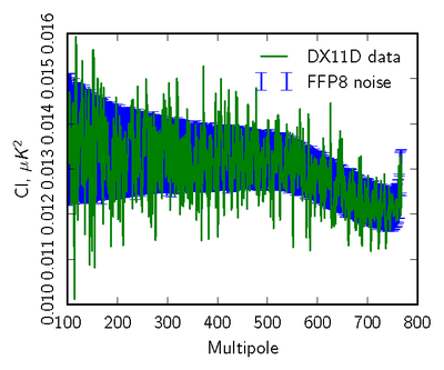
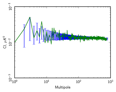
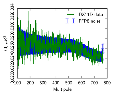
| + | [[File:null_cl_ffp8_070yr1+yr3-yr2+yr4_TT_log88mm.png|thumb|center|400px|'''Figure 2: Pseudo-spectrum comparison (70GHz <i>TT</i>) of 2-year data difference (Year(1+3)-Year(2+4) in green) to the FFP8 simulation distribution (blue error bars).''']] | ||
| + | |||
| + | [[File:null_cl_ffp8_070yr1+yr3-yr2+yr4_EE_lin_88mm.png|thumb|center|400px]] | ||
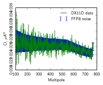
| + | [[File:null_cl_ffp8_070yr1+yr3-yr2+yr4_EE_log88mm.png|thumb|center|400px|'''Figure 3: Pseudo-spectrum comparison (70GHz <i>EE</i>) of 2-year data difference (Year(1+3)-Year(2+4) in green) to the FFP8 simulation distribution (blue error bars).''']] | ||
| + | |||
| + | [[File:null_cl_ffp8_070yr1+yr3-yr2+yr4_BB_lin_88mm.png|thumb|center|400px]] | ||
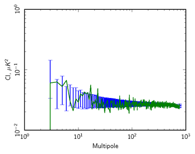
| + | [[File:null_cl_ffp8_070yr1+yr3-yr2+yr4_BB_log88mm.png|thumb|center|400px|'''Figure 4: Pseudo-spectrum comparison(70GHz <i>BB</i>) of 2-year data difference (Year(1+3)-Year(2+4) in green) to the FFP8 simulation distribution (blue error bars).''']] | ||
| + | |||
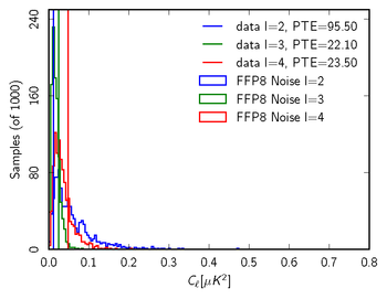
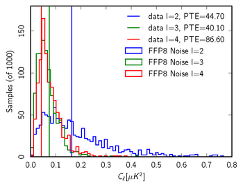
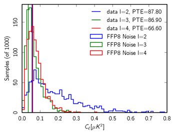
| + | Finally, we can look at the distribution of noise power from the Monte Carlos "ℓ by ℓ" and check where the real data fall in that distribution, to see if it is consistent with noise alone. | ||
| − | + | [[File:ffp8_dist_070full-survey_1survey_3_TT88mm_nt.png|350px|]] | |
| − | + | [[File:ffp8_dist_070full-survey_1survey_3_EE88mm_nt.png|350px|]] | |
| + | [[File:ffp8_dist_070full-survey_1survey_3_BB88mm_nt.png|350px|]] | ||
| + | '''<small>Figure 5: Sample 70GHz null test in comparison with FFP8 null distribution for multipoles from 2 to 4. From left to right we show <i>TT</i>, <i>EE</i>, <i>BB</i>. In this case, the null test is the full mission map - (Survey 1+Survey 3). We report the probability to exceed (PTE) values for the data relative to the FFP8 noise-only distributions. All values for this example are very reasonable, suggesting that our noise model captures the important features of the data even at low multipoles.</small>''' | ||
| − | |||
| − | |||
| − | |||
| − | |||
==Consistency checks == | ==Consistency checks == | ||
| − | All the details can be found in {{PlanckPapers|planck2013-p02}} {{PlanckPapers|planck2014-a03||Planck-2015-A03}}. | + | All the details of consistency tests performed can be found in {{PlanckPapers|planck2013-p02}} and {{PlanckPapers|planck2014-a03||Planck-2015-A03}}. |
| − | ===Intra frequency consistency check=== | + | ===Intra-frequency consistency check=== |
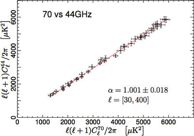
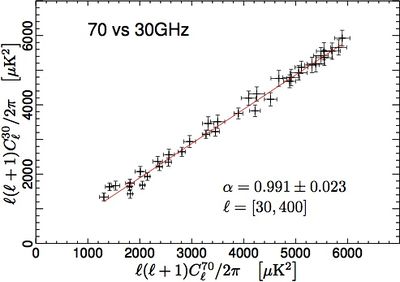
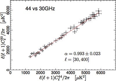
| − | We have tested the consistency between 30, 44, and | + | We have tested the consistency between 30, 44, and 70GHz maps by comparing the power spectra in the multipole range around the first acoustic peak. In order to do so, we have removed the estimated contribution from unresolved point source from the spectra. We have then built scatter plots for the three frequency pairs, i.e., 70GHz versus 30 GHz, 70GHz versus 44GHz, and 44GHz versus 30GHz, and performed a linear fit, accounting for errors on both axes. |
| − | The results reported in Fig. | + | The results reported in Fig. 6 show that the three power spectra are consistent within the errors. Moreover, note that the current error budget does not account for foreground removal, calibration, and window function uncertainties. Hence, the observed agreement between spectra at different frequencies can be considered to be even more satisfactory. |
| − | [[File:LFI_70vs44_DX11D_maskTCS070vs060_a.jpg|thumb|center|400px|]][[File:LFI_70vs30_DX11D_maskTCS070vs040_a.jpg|thumb|center|400px|]][[File:LFI_44vs30_DX11D_maskTCS060vs040_a.jpg|thumb|center|400px|'''Figure | + | [[File:LFI_70vs44_DX11D_maskTCS070vs060_a.jpg|thumb|center|400px|]][[File:LFI_70vs30_DX11D_maskTCS070vs040_a.jpg|thumb|center|400px|]][[File:LFI_44vs30_DX11D_maskTCS060vs040_a.jpg|thumb|center|400px|'''Figure 6: Consistency between spectral estimates at different frequencies. From top to bottom: 70GHz versus 44 GHz; 70GHz versus 30 GHz; and 44GHz versus 30 GHz. Solid red lines are the best fit of the linear regressions, whose angular coefficients α are consistent with unity within the errors.''']] |
===70 GHz internal consistency check=== | ===70 GHz internal consistency check=== | ||
| − | We use the Hausman test {{BibCite|polenta_CrossSpectra}} to assess the consistency of auto and cross spectral estimates at 70 GHz. We define the statistic: | + | We use the Hausman test {{BibCite|polenta_CrossSpectra}} to assess the consistency of auto- and cross-spectral estimates at 70 GHz. We specifically define the statistic: |
:<math> | :<math> | ||
| − | H_{\ell}=\left(\hat{C_{\ell}}-\tilde{C_{\ell}}\right)/\sqrt{Var\left\{ \hat{C_{\ell}}-\tilde{C_{\ell}}\right\} } | + | H_{\ell}=\left(\hat{C_{\ell}}-\tilde{C_{\ell}}\right)/\sqrt{{\rm Var}\left\{ \hat{C_{\ell}}-\tilde{C_{\ell}}\right\} }, |
</math> | </math> | ||
| − | where <math>\hat{C_{\ell}}</math> and <math>\tilde{C_{\ell}}</math> represent auto- and | + | where <math>\hat{C_{\ell}}</math> and <math>\tilde{C_{\ell}}</math> represent auto- and |
| − | cross-spectra respectively. In order to combine information from different multipoles into a single quantity, we define | + | cross-spectra, respectively. In order to combine information from different multipoles into a single quantity, we define |
:<math> | :<math> | ||
| − | B_{L}(r)=\frac{1}{\sqrt{L}}\sum_{\ell=2}^{[Lr]}H_{\ell},r\in\left[0,1\right] | + | B_{L}(r)=\frac{1}{\sqrt{L}}\sum_{\ell=2}^{[Lr]}H_{\ell},r\in\left[0,1\right], |
</math> | </math> | ||
| − | where | + | where square brackets denote the integer part. The distribution of <i>B<sub>L</sub></i>(<i>r</i>) |
converges (in a functional sense) to a Brownian motion process, which can be studied through the statistics | converges (in a functional sense) to a Brownian motion process, which can be studied through the statistics | ||
| − | < | + | <i>s</i><sub>1</sub>=sup<sub><i>r</i></sub><i>B<sub>L</sub></i>(<i>r</i>), |
| − | < | + | <i>s</i><sub>2</sub>=sup<sub><i>r</i></sub>|<i>B<sub>L</sub></i>(<i>r</i>)|, and |
| − | < | + | <i>s</i><sub>3</sub>=∫<sub>0</sub><sup>1</sup><i>B<sub>L</sub></i><sup>2</sup>(<i>r</i>)dr. Using the "FFP7" simulations, |
| − | we derive | + | we derive empirical distributions for all the three test statistics and compare with results obtained from Planck data |
| − | (see Fig. | + | (see Fig. 7). We find that the Hausman test shows no statistically significant inconsistencies between the two spectral |
estimates. | estimates. | ||
| − | [[File:cons2.jpg|thumb|center|800px|'''Figure | + | [[File:cons2.jpg|thumb|center|800px|'''Figure 7: From left to right, the empirical |
| − | distribution (estimated via | + | distribution (estimated via FFP7) of the <i>s</i><sub>1</sub>, <i>s</i><sub>2</sub>, and <i>s</i><sub>3</sub> |
| − | statistics (see text). The vertical line represents | + | statistics (see text). The vertical line represents 70GHz data.''']] |
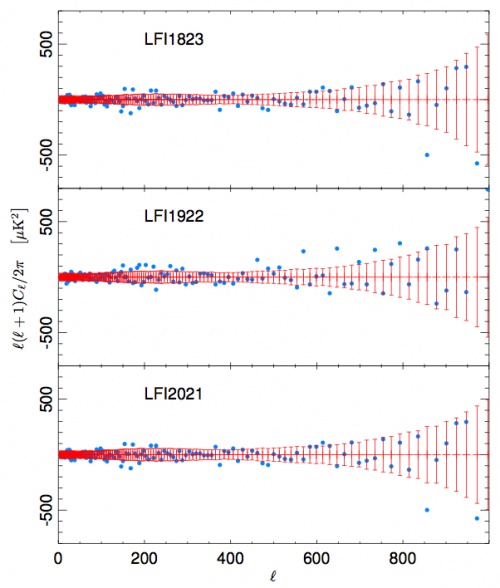
| − | As a further test, we have estimated the temperature power spectrum for each of three horn-pair | + | As a further test, we have estimated the temperature power spectrum for each of three horn-pair maps, and have compared the |
| − | results with the spectrum obtained from all | + | results with the spectrum obtained from all 12 radiometers shown above. In Fig. 8 we plot the |
difference between the horn-pair and the combined power spectra. | difference between the horn-pair and the combined power spectra. | ||
| − | Again, the error bars have been estimated from the | + | Again, the error bars have been estimated from the FFP7 simulated data set. A χ<sup>2</sup> analysis of the residual shows that they are compatible with the null hypothesis, confirming the |
strong consistency of the estimates. | strong consistency of the estimates. | ||
| − | [[File:cons3.jpg|thumb|center|500px|'''Figure | + | [[File:cons3.jpg|thumb|center|500px|'''Figure 8: Residuals between the auto-power spectra of the horn-pair maps and the power spectrum of the full 70GHz frequency map. Error bars here are derived from FFP7 simulations.''']] |
<!-- | <!-- | ||
Latest revision as of 13:37, 19 September 2016
Contents
Overview[edit]
Data validation is critical at each step of the analysis pipeline. Much of the LFI data validation is based on null tests. Here we present some examples from the current release, with comments on relevant time scales and sensitivity to various systematics.
Null tests approach[edit]
Null tests at map level are performed routinely, whenever changes are made to the mapmaking pipeline. These include differences at survey, year, 2-year, half- mission and half-ring levels, for single detectors, horns, horn pairs and full frequency complements. Where possible, map differences are generated in I, Q and U. For this release, we use the Full Focal Plane 8 (FFP8) simulations for comparison. We can use FFP8 noise simulations, identical to the data in terms of sky sampling and with matching time domain noise characteristics, to make statistical arguments about the likelihood of the noise observed in the actual data nulls. In general null tests are performed to highlight possible issues in the data related to instrumental systematic effecst not properly accounted for within the processing pipeline, or related to known changes in the operational conditions (e.g., switch-over of the sorption coolers), or related to intrinsic instrument properties coupled with the sky signal, such as stray light contamination. Such null-tests can be performed by using data on different time scales ranging from 1 minute to 1 year of observations, at different unit levels (radiometer, horn, horn-pair), within frequency and cross-frequency, both in total intensity, and, when applicable, in polarization.
Sample Null Maps[edit]
Figure 1: Null map samples for 30GHz (top), 44GHz (middle), and 70GHz (bottom). From left to right: half-ring differences in I and Q; 2-year combination differences in I and Q. All maps are smoothed to 3°.
Three things are worth pointing out generally about these maps.
Firstly, there are no obvious "features" standing out at this resolution and noise level. Earlier versions of the data processing, where there were errors in calibration for instance, would show scan-correlated structures at much larger amplitude.
Secondly, the half-ring difference maps and the 2-year combination difference maps give a very similar overall impression. This is a very good sign, as these two types of null map cover very different time scales (1 hour to 2 years).
Thirdly, it is impossible to know how "good" the test is just by looking at the map. There is clearly noise, but determining if it is consistent with the noise model of the instrument, and further, if it will bias the scientific results, requires more analysis.
Statistical Analyses[edit]
The next level of data compression is to use the angular power spectra of the null tests, and to compare to simulations in a statistically robust way. We use two different approaches. In the first we compare pseudo-spectra of the null maps to the half-ring spectra, which are the most "free" of anticipated systmatics. In the second, we use noise Monte Carlos from the FFP8 simulations, where we run the mapmaking identically to the real data, over data sets with identical sampling to the real data but consisting of noise only generated to match the per-detector LFI noise model.
Here we show examples comparing the pseudo-spectra of a set of 100 Monte Carlos to the real data. We mask both data and simlations to concentrate on residuals impacting CMB analyses away from the Galactic plane.
Finally, we can look at the distribution of noise power from the Monte Carlos "ℓ by ℓ" and check where the real data fall in that distribution, to see if it is consistent with noise alone.
Figure 5: Sample 70GHz null test in comparison with FFP8 null distribution for multipoles from 2 to 4. From left to right we show TT, EE, BB. In this case, the null test is the full mission map - (Survey 1+Survey 3). We report the probability to exceed (PTE) values for the data relative to the FFP8 noise-only distributions. All values for this example are very reasonable, suggesting that our noise model captures the important features of the data even at low multipoles.
Consistency checks[edit]
All the details of consistency tests performed can be found in Planck-2013-II[1] and Planck-2015-A03[2].
Intra-frequency consistency check[edit]
We have tested the consistency between 30, 44, and 70GHz maps by comparing the power spectra in the multipole range around the first acoustic peak. In order to do so, we have removed the estimated contribution from unresolved point source from the spectra. We have then built scatter plots for the three frequency pairs, i.e., 70GHz versus 30 GHz, 70GHz versus 44GHz, and 44GHz versus 30GHz, and performed a linear fit, accounting for errors on both axes. The results reported in Fig. 6 show that the three power spectra are consistent within the errors. Moreover, note that the current error budget does not account for foreground removal, calibration, and window function uncertainties. Hence, the observed agreement between spectra at different frequencies can be considered to be even more satisfactory.
70 GHz internal consistency check[edit]
We use the Hausman test [3] to assess the consistency of auto- and cross-spectral estimates at 70 GHz. We specifically define the statistic:
where and represent auto- and cross-spectra, respectively. In order to combine information from different multipoles into a single quantity, we define
where square brackets denote the integer part. The distribution of BL(r) converges (in a functional sense) to a Brownian motion process, which can be studied through the statistics s1=suprBL(r), s2=supr|BL(r)|, and s3=∫01BL2(r)dr. Using the "FFP7" simulations, we derive empirical distributions for all the three test statistics and compare with results obtained from Planck data (see Fig. 7). We find that the Hausman test shows no statistically significant inconsistencies between the two spectral estimates.
As a further test, we have estimated the temperature power spectrum for each of three horn-pair maps, and have compared the results with the spectrum obtained from all 12 radiometers shown above. In Fig. 8 we plot the difference between the horn-pair and the combined power spectra. Again, the error bars have been estimated from the FFP7 simulated data set. A χ2 analysis of the residual shows that they are compatible with the null hypothesis, confirming the strong consistency of the estimates.
References[edit]
- ↑ Planck 2013 results. II. Low Frequency Instrument data processing, Planck Collaboration, 2014, A&A, 571, A2
- ↑ Planck 2015 results. II. LFI processing, Planck Collaboration, 2016, A&A, 594, A2.
- ↑ Unbiased estimation of an angular power spectrum, G. Polenta, D. Marinucci, A. Balbi, P. de Bernardis, E. Hivon, S. Masi, P. Natoli, N. Vittorio, J. Cosmology Astropart. Phys., 11, 1, (2005).
(Planck) Low Frequency Instrument
Cosmic Microwave background
[LFI meaning]: absolute calibration refers to the 0th order calibration for each channel, 1 single number, while the relative calibration refers to the component of the calibration that varies pointing period by pointing period.


