CMB and astrophysical component maps
Contents
Overview[edit]
This section describes the maps of astrophysical components produced from the Planck data. These products are derived from some or all of the nine frequency channel maps described above using different techniques and, in some cases, using other constraints from external data sets. Here we give a brief description of the product and how it is obtained, followed by a description of the FITS file containing the data and associated information. All the details can be found in #planck2013-p06.
CMB maps[edit]
Four pipelines have been used to produce maps of the CMB: Commander-Ruler, NILC, SEVEM and SMICA. The last three have been delivered as Legacy Archive products.
The front-runner CMB map is the SMICA one. This product is labeled as "Main product" in the Planck Legacy Archive Java interface while the two others (NILC, SEVEM) are labeled as "Additional product".
The component separation pipelines are described in the CMB and foreground separation section and also in Section 3 and Appendices A-D of #planck2013-p06 Planck-2013-XII and references therein.
Product description[edit]
- SMICA
SMICA produces a CMB map by linearly combining all Planck input channels (from 30 to 857 GHz) with weights which vary with the multipole.
The SMICA map has an effective beam window function of 5 arc-minutes, deconvolved from the pixel window. It means that, ideally, one would have , where is the angular spectrum of the map, where is the angular spectrum of the CMB and is a 5-arcminute Gaussian beam function.
The SMICA map has been inpainted over 3% of the sky using a constrained Gaussian realisation. A binary mask describing the inpainted area is provided.
We provide a confidence mask which excludes some parts of the Galactic plane and also the masked point sources.
- NILC
Needlet-ILC (hereafter NILC) produces a CMB map by applying the Internal Linear Combination (ILC) technique in needlet space, that is, with combination weights which are allowed to vary over the sky and over the whole multipole range.
It uses all Planck channels from 44 to 857 GHz.
- SEVEM
The aim of SEVEM is to produce clean CMB maps at one or several frequencies by using a procedure based on template fitting. The templates are internal, i.e., they are constructed from Planck data, avoiding the need for external data sets, which usually complicates the analyses and may introduce inconsistencies. The method has been successfully applied to Planck simulations Leach et al., 2008 #leach2008 and to WMAP polarisation data Fernandez-Cobos et al., 2012 xx. In the cleaning process, no assumptions about the foregrounds or noise levels are needed, rendering the technique very robust.
Production process[edit]
- SMICA
The actual implementation of SMICA includes the following steps:
- Inputs
- All nine Planck frequency channels from 30 to 857 GHz, harmonically transformed up to .
- Fit
- In practice, the SMICA fit,i.e.,the minimization of Eq. (4) in the SMICA description section, is conducted in three successive steps: We first estimate the CMB spectral law by fitting all model parameters over a clean fraction of sky in the range and retaining the best fit value for vector . In the second step, we estimate the foreground emissivity by fixing a to its value from the previous step and fitting all the other parameters over a large fraction of sky in the range and retaining the best fit values for the matrix . In the last step, we fit all power spectrum parameters; that is, we fix and to their previously found values and fit for each and at each .
- Beams
- The discussion thus far assumes that all input maps have the same resolution and effective beam. Since the observed maps actually vary in resolution, we process the input maps in the following way. To the -th input map with effective beam and sampled on an HEALPix grid with , the CMB sky multipole actually contributes , where is the pixel window function for the grid at . Seeking a final CMB map at 5-arcmin resolution, the highest resolution of Planck, we work with input spherical harmonics re-beamed to 5 arcmins, ; that is, SMICA operates on vectors with entries , where is a 5 arcmin Gaussian beam function. By construction, SMICA then produces an CMB map with an effective Gaussian beam of 5 arcmin (without the pixel window function).
- Pre-processing
- We start by fitting point sources with SNR > 5 in the PCCS catalogue in each input map. If the fit is successful, the fitted point source is removed from the map; otherwise it is masked and the hole in-painted. This is done at all frequencies but 545 and 857 GHz, where all point sources with SNR > 7.5 are masked and in-painted.
- Masking and in-painting
- In practice, SMICA uses a small Galactic mask leaving 97% of the sky. We deliver a full-sky CMB map in which the masked pixels (Galactic and point-source) are replaced by a constrained Gaussian realization.
- Binning
- In our implementation, we use binned spectra.
- High
- Since there is little point trying to model the spectral covariance at high multipoles, because the sample estimate is sufficient, SMICA implements a simple harmonic ILC at ; that is, it applies the filter (Eq. (2) in the SMICA description section) with .
Viewed as a filter, SMICA can be summarized by the weights applied to each input map as a function of multipole. In this sense, SMICA is strictly equivalent to co-adding the input maps after convolution by specific axi-symmetric kernels directly related to the corresponding entry of . The SMICA weights used here are shown in the figure below for input maps in units of K. They show, in particular, the (expected) progressive attenuation of the lowest resolution channels with increasing multipole.

- NILC
The ability linearly to combine input maps varying over the sky and over multipoles is called ‘localisation’. In the needlet framework, harmonic localisation is achieved using a set of bandpass filters defining ‘scales’ and spatial localization is achieved, at each scale, by defining zones over the sky. The harmonic localisation used here uses 9 spectral bands covering multipoles up to = 3200 (see figure below). The spatial localisation depends on the scale: at the coarsest scale, which include the multipoles of lowest degree, we use a single zone (no localization) while at the finest scales (which include the highest degree multipoles), the sky is partitioned in up to 20 zones (again, see figure below).
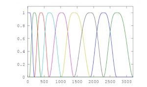
Spectral window functions defining nine needlet scales
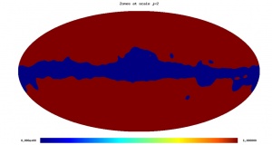
The 2-zone partition
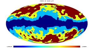
The 4-zone partition
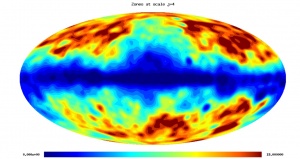
The 20-zone partition.


Spectral localization for NILC using with nine spectral window functions defining nine ‘needlet scales’ (top left panel). The scale-dependent spatial localization partitions the sky in 1 zone (for scale 1), 2 zones (for scale 2), 4 zones (for scale 3), or 20 zones (for scales 5, 6, 7, 8, 9).
The NILC method amounts to applying an ILC in each zone of each scale, allowing the ILC weights to adapt naturally to the varying strength of the contaminants as a function of direction and multipole. A complete description of the basic NILC method can be found in Delabrouille et al. (2009) #delabrouille2009. In this work, however, we have implemented an important difference for the processing of the coarsest scale.
The actual processing differs from the above scenario in several respects: pre-processing of point sources, dealing with frequency-dependent beams, and dealing with statistical issues (the ILC bias) in the coarsest scale.
- Pre-processing of point sources. Identical to the SMICA pre-processing.
- Masking and inpainting. The NILC CMB map is actually produced in a two step process. In a first step, the NILC weights are computed from needlet statistics evaluated using a Galactic mask which covers about 98% of the sky (and is apodiwed at 1 degree). In a second step, those NILC weights on are applied to needlet coefficients computed over the whole sky (the point sources having been subtracted or fitted at the pre-processing stage), yielding a NILC CMB estimate over the whole sky, except for the point source mask. In a final step, those masked pixels are replaced by the values of a constrained Gaussian realization.
- Beam control and transfer function. As in the SMICA processing (see that section), the input maps are represented by their spherical harmonic coefficients. By internally rebeaming to a 5 arcmin resolution and by the unbiasedness property of the ILC, the resulting CMB map is automatically synthesized with an effective Gaussian beam of 5 arcmin.
- ILC bias and spectral statistics for the coarsest scale. The coarsest scale of the NILC filter is not localized. Therefore, the NILC map at the coarsest scale is equivalent to a plain pixel-based ILC which is known to be quite susceptible to an ‘ILC bias’ due to chance correlations between the CMB and foregrounds. In order to mitigate that effect, the covariance matrix which determines the ILC coefficients at the coarsest scale is not computed as a pixel average but is rather estimated in the spectral domain with a spectral weight which equalizes the power of the CMB modes (based on a fiducial spectrum).
- Using SMICA recalibration. In our current rendering, the NILC uses for the CMB emission law the values determined by SMICA.
- SEVEM
The templates are internal, i.e., they are constructed from Planck data, avoiding the need for external data sets, which usually complicates the analyses and may introduce inconsistencies. In the cleaning process, no assumptions about the foregrounds or noise levels are needed, rendering the technique very robust. The fitting can be done in real or wavelet space (using a fast wavelet adapted to the HEALPix pixelization; Casaponsa et al. 2011 #Casaponsa2011) to properly deal with incomplete sky coverage. By expediency, however, we fill in the small number of unobserved pixels at each channel with the mean value of its neighbouring pixels before applying SEVEM.
We construct our templates by subtracting two close Planck frequency channel maps, after first smoothing them to a common resolution to ensure that the CMB signal is properly removed. A linear combination of the templates is then subtracted from (hitherto unused) map d to produce a clean CMB map at that frequency. This is done either in real or in wavelet space (i.e., scale by scale) at each position on the sky:
where is the number of templates. If the cleaning is performed in real space, the coefficients are obtained by minimising the variance of the clean map outside a given mask. When working in wavelet space, the cleaning is done in the same way at each wavelet scale independently (i.e., the linear coefficients depend on the scale). Although we exclude very contaminated regions during the minimization, the subtraction is performed for all pixels and, therefore, the cleaned maps cover the full-sky (although we expect that foreground residuals are present in the excluded areas).
An additional level of flexibility can also be considered: the linear coefficients can be the same for all the sky, or several regions with different sets of coefficients can be considered. The regions are then combined in a smooth way, by weighting the pixels at the boundaries, to avoid discontinuities in the clean maps. Since the method is linear, we may easily propagate the noise properties to the final CMB map. Moreover, it is very fast and permits the generation of thousands of simulations to character- ize the statistical properties of the outputs, a critical need for many cosmological applications. The final CMB map retains the angular resolution of the original frequency map.
There are several possible configurations of SEVEM with regard to the number of frequency maps which are cleaned or the number of templates that are used in the fitting. Note that the production of clean maps at different frequencies is of great interest in order to test the robustness of the results. Therefore, to define the best strategy, one needs to find a compromise between the number of maps that can be cleaned independently and the number of templates that can be constructed.
In particular, we have cleaned the 143 GHz and 217 GHz maps using four templates constructed as the difference of the following Planck channels (smoothed to a common resolution): (30-44), (44-70), (545-353) and (857-545). For simplicity, the three maps have been cleaned in real space, since there was not a significant improvement when using wavelets (especially at high latitude). In order to take into account the different spectral behaviour of the foregrounds at low and high galactic latitudes, we have considered two independent regions of the sky, for which we have used a different set of coefficients. The first region corresponds to the 3 per cent brightest Galactic emission, whereas the second region is defined by the remaining 97 per cent of the sky. For the first region, the coefficients are actually estimated over the whole sky (we find that this is more optimal than perform the minimisation only on the 3 per cent brightest region, where the CMB emission is very sub-dominant) while for the second region, we exclude the 3 per cent brightest region of the sky, point sources detected at any frequency and those pixels which have not been observed at all channels. Our final CMB map has then been constructed by combining the 143 and 217 GHz maps by weighting the maps in harmonic space taking into account the noise level, the resolution and a rough estimation of the foreground residuals of each map (obtained from realistic simulations). This final map has a resolution corresponding to a Gaussian beam of fwhm=5 arcminutes.
Moreover, additional CMB clean maps (at frequencies between 44 and 353 GHz) have also been produced using different combinations of templates for some of the analyses carried out in #planck2013-p09 Planck-2013-XXIII and #planck2013-p14 Planck-2013-XIX . In particular, clean maps from 44 to 353 GHz have been used for the stacking analysis presented in #planck2013-p14, while frequencies from 70 to 217 GHz were used for consistency tests in #planck2013-p09.
The method has been successfully applied to Planck simulations #leach2008 and to WMAP polarisation data #Fernandez-Cobos2012.
Inputs[edit]
The input maps are the sky temperature maps described in the Sky temperature maps section.
- SMICA
SMICA uses all nine Planck frequency channels from 30 to 857 GHz. SMICA uses a pre-processing step in which point sources are subtracted or masked as described above.
- NILC
NILC uses eight frequency channels from 44 to 857 GHz and the same pre-processing step as SMICA.
- SEVEM
SEVEM uses all nine Planck frequency channel maps. The 30 - 70 GHz and 353 - 857 GHz maps are used to construct templates by taking the differences (30 - 44) GHz, (44 - 70) GHz, (545 - 353) GHz and (857 - 545) GHz, after smoothing to a common resolution. The 100, 143 and 217 GHz maps are cleaned using the templates.
File names and structure[edit]
The FITS files corresponding to the three CMB products are the following:
- COM_CompMap_CMB-nilc_2048_R1.11.fits
- COM_CompMap_CMB-sevem_2048_R1.11.fits
- COM_CompMap_CMB-smica_2048_R1.11.fits
and the CMB they contain is shows below.

SMICA
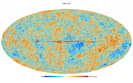
NILC
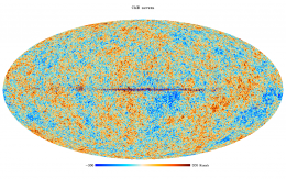
SEVEM


The files contains a minimal primary extension with no data and four data extensions which are described in the table below:
| Ext. 1. EXTNAME = COMP-MAP (BINTABLE) | |||
|---|---|---|---|
| Column Name | Data Type | Units | Description |
| I | Real*4 | uK_cmb | The CMB temperature map |
| NOISE | Real*4 | uK_cmb | Estimated noise map (Note 1) |
| VALMASK | Byte | none | Validity, or confidence mask (note 2) |
| INPMASK | Byte | none | Inpainted mask (Optional - see Note 3) |
| Keyword | Data Type | Value | Description |
| AST-COMP | String | CMB | Astrophysical compoment name |
| PIXTYPE | String | HEALPIX | |
| COORDSYS | String | GALACTIC | Coordinate system |
| ORDERING | String | NESTED | Healpix ordering |
| NSIDE | Int | 2048 | Healpix Nside |
| METHOD | String | name | Cleaning method (SMICA/NILC/SEVEM) |
| Ext. 2. EXTNAME = FGDS-LFI (BINTABLE) - Note 4 | |||
| Column Name | Data Type | Units | Description |
| LFI_030 | Real*4 | K_cmb | 30 GHz foregrounds |
| LFI_044 | Real*4 | K_cmb | 44 GHz foregrounds |
| LFI_070 | Real*4 | K_cmb | 70 GHz foregrounds |
| Keyword | Data Type | Value | Description |
| PIXTYPE | String | HEALPIX | |
| COORDSYS | String | GALACTIC | Coordinate system |
| ORDERING | String | NESTED | Healpix ordering |
| NSIDE | Int | 1024 | Healpix Nside |
| METHOD | String | name | Cleaning method (SMICA/NILC/SEVEM) |
| Ext. 3. EXTNAME = FGDS-HFI (BINTABLE) - Note 4 | |||
| Column Name | Data Type | Units | Description |
| HFI_100 | Real*4 | K_cmb | 100 GHz foregrounds |
| HFI_143 | Real*4 | K_cmb | 143 GHz foregrounds |
| HFI_217 | Real*4 | K_cmb | 217 GHz foregrounds |
| HFI_353 | Real*4 | K_cmb | 353 GHz foregrounds |
| HFI_545 | Real*4 | MJy/sr | 545 GHz foregrounds |
| HFI_857 | Real*4 | MJy/sr | 857 GHz foregrounds |
| Keyword | Data Type | Value | Description |
| PIXTYPE | String | HEALPIX | |
| COORDSYS | String | GALACTIC | Coordinate system |
| ORDERING | String | NESTED | Healpix ordering |
| NSIDE | Int | 2048 | Healpix Nside |
| METHOD | String | name | Cleaning method (SMICA/NILC/SEVEM) |
| Ext. 4. EXTNAME = BEAM_WF (BINTABLE) | |||
| Column Name | Data Type | Units | Description |
| BEAM_WF | Real*4 | uK_cmb | The CMB temperature map |
| Keyword | Data Type | Value | Description |
| LMIN | Int | value | First multipole of beam WF |
| LMAX | Int | value | Lsst multipole of beam WF |
| METHOD | String | name | Cleaning method (SMICA/NILC/SEVEM) |
Notes:
- The half-ring half-difference (HRHD) map is made by passing the half-ring frequency maps independently through the component separation pipeline, then computing half their difference. It approximates a noise realisation, and gives an indication of the uncertainties due to instrumental noise in the corresponding CMB map.
- The confidence mask indicates where the CMB map is considered valid.
- NILC and SMICA CMB maps have been inpainted in the Galactic plane and around some bright sources with a constrained realisation of the signal. The inpainted area covers approximately 3% of the sky. This column is not present in the SEVEM product file.
- The subtraction of the CMB from the sky maps in order to produce the foregrounds map is done after convolving the CMB map to the resolution of the given frequency.
Cautionary notes[edit]
- The half-ring CMB maps are produced by the pipelines with parameters/weights fixed to the values obtained from the full maps. Therefore the CMB HRHD maps do not capture all of the uncertainties due to foreground modelling on large angular scales.
- The HRHD maps for the HFI frequency channels underestimate the noise power spectrum at high l by typically a few percent. This is caused by correlations induced in the pre-processing to remove cosmic ray hits. The CMB is mostly constrained by the HFI channels at high l, and so the CMB HRHD maps will inherit this deficiency in power.
- The beam transfer functions do not account for uncertainties in the beams of the frequency channel maps.
Astrophysical foregrounds from parametric component separation[edit]
We describe diffuse foreground products for the Planck 2013 release. See Planck Component Separation paper #planck2013-p06 Planck-2013-XII for a detailed description and astrophysical discussion of those.
Product description[edit]
- Low frequency foreground component
- The products below contain the result of the fitting for one foreground component at low frequencies in Planck bands,along with its spectral behavior parametrized by a power law spectral index. Amplitude and spectral indeces are evaluated at N$_\rm{side}$ 256 (see below in the production process), along with standard deviation from sampling and instrumental noise on both. An amplitude solution at N$_\rm{side}$=2048 is also given, along with standard deviation from sampling and instrumental noise as well as solutions on halfrings. The beam profile associated to this component is also provided as a secondary Extension in the N$_\rm{side}$ 2048 product.
- Thermal dust
- The products below contain the result of the fitting for one foreground component at high frequencies in Planck bands, along with its spectral behavior parametrized by temperature and emissivity. Amplitude, temperature and emissivity are evaluated at N$_\rm{side}$ 256 (see below in the production process), along with standard deviation from sampling and instrumental noise on all of them. An amplitude solution at N$_\rm{side}$=2048 is also given, along with standard deviation from sampling and instrumental noise as well as solutions on halfrings. The beam profile associated to this component is provided.
- Sky mask
- The delivered mask is defined as the sky region where the fitting procedure was conducted and the solutions presented here were obtained. It is made by masking a region where the Galactic emission is too intense to perform the fitting, plus the masking of brightest point sources.
Production process[edit]
CODE: COMMANDER-RULER. The code exploits a parametrization of CMB and main diffuse foreground observables. The naive resolution of input frequency channels is reduced to N$_\rm{side}$=256 first. Parameters related to the foreground scaling with frequency are estimated at that resolution by using Markov Chain Monte Carlo analysis using Gibbs sampling. The foreground parameters make the foreground mixing matrix which is applied to the data at full resolution in order to obtain the provided products at N$_\rm{side}$=2048. In the Planck Component Separation paper #planck2013-p06 Planck-2013-XII additional material is discussed, specifically concerning the sky region where the solutions are reliable, in terms of chi2 maps.
Inputs[edit]
Nominal frequency maps at 30, 44, 70, 100, 143, 217, 353 GHz (LFI 30 GHz frequency maps, LFI 44 GHz frequency maps and LFI 70 GHz frequency maps, HFI 100 GHz frequency maps, HFI 143 GHz frequency maps,HFI 217 GHz frequency maps and HFI 353 GHz frequency maps) and their II column corresponding to the noise covariance matrix. Halfrings at the same frequencies. Beam window functions as reported in the LFI and HFI RIMO.
Related products[edit]
None.
File names[edit]
- Low frequency component at N$_\rm{side}$ 256:
- Low frequency component at N$_\rm{side}$ 2048:
- Thermal dust at N$_\rm{side}$ 256:
- Thermal dust at N$_\rm{side}$ 2048:
- Mask:
Meta Data[edit]
Low frequency foreground component[edit]
Low frequency component at N$_\rm{side}$ 256[edit]
File name: COM_CompMap_Lfreqfor-commrul_0256_R1.00.fits
- Name HDU -- COMP-MAP
The Fits extension is composed by the columns described below:
| Column Name | Data Type | Units | Description |
|---|---|---|---|
| I | Real*4 | uK | Intensity |
| I_stdev | Real*4 | uK | standard deviation of intensity |
| Beta | Real*4 | effective spectral index | |
| B_stdev | Real*4 | standard deviation on the effective spectral index |
- Notes
- Comment: The Intensity is normalized at 30 GHz
- Comment: The intensity was estimated during mixing matrix estimation
Below an example of the header.
Low frequency component at N$_\rm{side}$ 2048[edit]
- File name: COM_CompMap_Lfreqfor-commrul_2048_R1.00.fits
- Name HDU -- COMP-MAP
The Fits extension is composed by the columns described below:
| Column Name | Data Type | Units | Description |
|---|---|---|---|
| I | Real*8 | uK | Intensity |
| I_stdev | Real*8 | uK | standard deviation of intensity |
| I_hr1 | Real*8 | uK | Intensity on half ring 1 |
| I_hr2 | Real*8 | uK | Intensity on half ring 2 |
- Notes
- Comment: The intensity was computed after mixing matrix application
- Name HDU -- BeamWF
The Fits second extension is composed by the columns described below:
| Column Name | Data Type | Units | Description |
|---|---|---|---|
| BeamWF | Real*4 | beam profile |
- Notes
- Comment: Beam window function used in the Component separation process
Below an example of the header of the first and second extension respectively.
Thermal dust[edit]
Thermal dust component at N$_\rm{side}$=256[edit]
- File name: COM_CompMap_dust-commrul_0256_R1.00.fits
- Name HDU -- COMP-MAP
The Fits extension is composed by the columns described below:
| Column Name | Data Type | Units | Description |
|---|---|---|---|
| I | Real*4 | MJy/sr | Intensity |
| I_stdev | Real*4 | MJy/sr | standard deviation of intensity |
| Em | Real*4 | emissivity | |
| Em_stdev | Real*4 | standard deviation on emissivity | |
| T | Real*4 | uK | temperature |
| T_stdev | Real*4 | uK | standard deviation on temerature |
- Notes
- Comment: The intensity is normalized at 353 GHz
Below an example of the header.
Thermal dust component at N$_\rm{side}$=2048[edit]
File name: COM_CompMap_dust-commrul_2048_R1.00.fits
- Name HDU -- COMP-MAP
The Fits extension is composed by the columns described below:
| Column Name | Data Type | Units | Description |
|---|---|---|---|
| I | Real*8 | MJy/sr | Intensity |
| I_stdev | Real*8 | MJy/sr | standard deviation of intensity |
| I_hr1 | Real*8 | MJy/sr | Intensity on half ring 1 |
| I_hr2 | Real*8 | MJy/sr | Intensity on half ring 2 |
- Name HDU -- BeamWF
The Fits second extension is composed by the columns described below:
| Column Name | Data Type | Units | Description |
|---|---|---|---|
| BeamWF | Real*4 | beam profile |
- Notes
- Comment: Beam window function used in the Component separation process
Below an example of the header of the first and second extension respectively.
Sky mask[edit]
File name: COM_CompMap_Mask-rulerminimal_2048.fits
- Name HDU -- COMP-MASK
The Fits extension is composed by the columns described below:
| Column Name | Data Type | Units | Description |
|---|---|---|---|
| Mask | Real*4 | Mask |
Below an example of the header.
Dust optical depth map and model[edit]
Thermal emission from interstellar dust is captured by Planck-HFI over the whole sky, at all frequencies from 100 to 857 GHz. This emission is well modelled by a modified black body in the far-infrared to millimeter range. It is produced by the biggest interstellar dust grain that are in thermal equilibrium with the radiation field from stars. The grains emission properties in the sub-millimeter are therefore directly linked to their absorption properties in the UV-visible range. By modelling the thermal dust emission in the sub-millimeter, a map of dust reddening in the visible can then be constructed.
- Model of thermal dust emission
The model of the thermal dust emission is based on a modify black body fit to the data $I_\nu$
$I_\nu = A\, B_\nu(T)\, \nu^\beta$
where B_nu(T) is the Planck function for dust equilibirum temperature T, A is the amplitude of the MBB and beta the dust spectral index. The dust optical depth at frequency nu is
$\tau_\nu = I_\nu / B_\nu(T) = A\, \nu^\beta$
The dust parameters provided are $T$, beta and $\tau_{353}$. They were obtained by fitting the Planck data at 353, 545 and 857 GHz together with the IRAS (IRIS) 100 micron data. All maps (in Healpix N$_\rm{side}$=2048) were smoothed to a common resolution of 5 arcmin. The CMB anisotropies, clearly visible at 353 GHz, were removed from all the HFI maps using the SMICA map. An offset was removed from each map to obtained a meaningful Galactic zero level, using a correlation with the LAB 21 cm data in diffuse areas of the sky ($N_{HI} < 2\times10^{20} cm^{-2}$). Because the dust emission is so well correlated between frequencies in the Rayleigh-Jeans part of the dust spectrum, the zero level of the 545 and 353 GHz were improved by correlating with the 857 GHz over a larger mask ($N_{HI} < 3\times10^{20} cm^{-2}$). Faint residual dipole structures, identified in the 353 and 545 GHz maps, were removed prior to the fit.
The MBB fit was performed using a chi-square minimization, assuming errors for each data point that include instrumental noise, calibration uncertainties (on both the dust emission and the CMB anisotropies) and uncertainties on the zero level. Because of the known degeneracy between $T$ and $\beta$ in the presence of noise, we produced a model of dust emission using data smoothed to 35 arcmin; at such resolution no systematic bias of the parameters is observed. The map of the spectral index $\beta$ at 35 arcmin was than used to fit the data for $T$ and $\tau_{353}$ at 5 arcmin.
- The $E(B-V)$ map
For the production of the $E(B-V)$ map, we used Planck and IRAS data from which point sources in diffuse areas were removed to avoid contamination by galaxies. In the hypothesis of constant dust emission cross-section, the optical depth map $\tau_{353}$ is proportional to dust column density. It can then be used to estimate E(B-V), also proportional to dust column density in the hypothesis of a constant differential absorption cross-section between the B and V bands. Given those assumptions, $ E(B-V) = q\, \tau_{353}$.
To estimate the calibration factor q, we followed a method similar to #mortsell2013 based on SDSS reddening measurements ($E(g-r)$ which corresponds closely to $E(B-V)$) of 77 429 Quasars #schneider2007. The interstellar HI column densities covered on the lines of sight of this sample ranges from $0.5$ to $10\times10^{20}\,cm^{-2}$. Therefore this sample allows to estimate q in the diffuse ISM where dust properties are expected to vary less than in denser clouds where coagulation and grain growth might modify dust emission and absorption cross sections.
- Dust optical depth products
The characteristics of the dust model maps are the following.
- Dust optical depth at 353 GHz : N$_\rm{side}$=2048, fwhm=5 arcmin, no units
- Dust reddening E(B-V) : N$_\rm{side}$=2048, fwhm=5 arcmin, units=magnitude, obtained with data from which point sources were removed.
- Dust temperature : N$_\rm{side}$ 2048, fwhm=5 arcmin, units=Kelvin
- Dust spectral index : N$_\rm{side}$=2048, fwhm=35 arcmin, no units
| 1. EXTNAME = 'COMP-MAP' | |||
|---|---|---|---|
| Column Name | Data Type | Units | Description |
| TAU353 | Real*4 | none | The opacity at 353GHz |
| TAU353ERR | Real*4 | none | Error in the opacity |
| EBV | Real*4 | mag | E(B-V) |
| EBV_ERR | Real*4 | mag | Error in E(B-V) |
| T_HF | Real*4 | K | Temperature for the high frequency correction |
| T_HF_ERR | Real*4 | K | Error on the temperature |
| BETAHF | Real*4 | none | Beta for the high frequency correction |
| BETAHFERR | Real*4 | none | Error on beta |
| Keyword | Data Type | Value | Description |
| AST-COMP | String | DUST-OPA | Astrophysical compoment name |
| PIXTYPE | String | HEALPIX | |
| COORDSYS | String | GALACTIC | Coordinate system |
| ORDERING | String | NESTED | Healpix ordering |
| NSIDE | Int | 2048 | Healpix N$_\rm{side}$ for LFI and HFI, respectively |
| FIRSTPIX | Int*4 | 0 | First pixel number |
| LASTPIX | Int*4 | 50331647 | Last pixel number, for LFI and HFI, respectively |
CO emission maps[edit]
CO rotational transition line emission is present in all HFI bands but for the 143 GHz channel. It is especially significant in the 100, 217 and 353 GHz channels (due to the 115 (1-0), 230 (2-1) and 345 GHz (3-2) CO transitions). This emission comes essentially from the Galactic interstellar medium and is mainly located at low and intermediate Galactic latitudes. Three approaches (summarised below) have been used to extract CO velocity-integrated emission maps from HFI maps and to make three types of CO products. An introduction is given in Section and a full description of these products is given in #planck2013-p03a.
- Type 1 product: it is based on a single channel approach using the fact that each CO line has a slightly different transmission in each bolometer at a given frequency channel. These transmissions can be evaluated from bandpass measurements that were performed on the ground or empirically determined from the sky using existing ground-based CO surveys. From these, the J=1-0, J=2-1 and J=3-2 CO lines can be extracted independently. As this approach is based on individual bolometer maps of a single channel, the resulting Signal-to-Noise ratio (SNR) is relatively low. The benefit, however, is that these maps do not suffer from contamination from other HFI channels (as is the case for the other approaches) and are more reliable, especially in the Galactic Plane.
- Type 2 product: this product is obtained using a multi frequency approach. Three frequency channel maps are combined to extract the J=1-0 (using the 100, 143 and 353 GHz channels) and J=2-1 (using the 143, 217 and 353 GHz channels) CO maps. Because frequency channels are combined, the spectral behaviour of other foregrounds influences the result. The two type 2 CO maps produced in this way have a higher SNR than the type 1 maps at the cost of a larger possible residual contamination from other diffuse foregrounds.
- Type 3 product: using prior information on CO line ratios and a multi-frequency component separation method, we construct a combined CO emission map with the largest possible SNR. This type 3 product can be used as a sensitive finder chart for low-intensity diffuse CO emission over the whole sky.
The released Type 1 CO maps have been produced using the MILCA-b algorithm, Type 2 maps using a specific implementation of the Commander algorithm, and the Type 3 map using the full Commander-Ruler component separation pipeline (see above).
Characteristics of the released maps are the following. We provide Healpix maps with N$_\rm{side}$=2048. For one transition, the CO velocity-integrated line signal map is given in K_RJ.km/s units. A conversion factor from this unit to the native unit of HFI maps (K_CMB) is provided in the header of the data files and in the RIMO. Four maps are given per transition and per type:
- The signal map
- The standard deviation map (same unit as the signal),
- A null test noise map (same unit as the signal) with similar statistical properties. It is made out of half the difference of half-ring maps.
- A mask map (0B or 1B) giving the regions (1B) where the CO measurement is not reliable because of some severe identified foreground contamination.
All products of a given type belong to a single file. Type 1 products have the native HFI resolution i.e. approximately 10, 5 and 5 arcminutes for the CO 1-0, 2-1, 3-2 transitions respectively. Type 2 products have a 15 arcminute resolution The Type 3 product has a 5.5 arcminute resolution.
| 1. EXTNAME = 'COMP-MAP' | |||
|---|---|---|---|
| Column Name | Data Type | Units | Description |
| I10 | Real*4 | K_RJ km/sec | The CO(1-0) intensity map |
| E10 | Real*4 | K_RJ km/sec | Uncertainty in the CO(1-0) intensity |
| N10 | Real*4 | K_RJ km/sec | Map built from the half-ring difference maps |
| M10 | Byte | none | Region over which the CO(1-0) intensity is considered reliable |
| I21 | Real*4 | K_RJ km/sec | The CO(2-1) intensity map |
| E21 | Real*4 | K_RJ km/sec | Uncertainty in the CO(2-1) intensity |
| N21 | Real*4 | K_RJ km/sec | Map built from the half-ring difference maps |
| M21 | Byte | none | Region over which the CO(2-1) intensity is considered reliable |
| I32 | Real*4 | K_RJ km/sec | The CO(3-2) intensity map |
| E32 | Real*4 | K_RJ km/sec | Uncertainty in the CO(3-2) intensity |
| N32 | Real*4 | K_RJ km/sec | Map built from the half-ring difference maps |
| M32 | Byte | none | Region over which the CO(3-2) intensity is considered reliable |
| Keyword | Data Type | Value | Description |
| AST-COMP | string | CO-TYPE2 | Astrophysical compoment name |
| PIXTYPE | String | HEALPIX | |
| COORDSYS | String | GALACTIC | Coordinate system |
| ORDERING | String | NESTED | Healpix ordering |
| NSIDE | Int | 2048 | Healpix N$_\rm{side}$ for LFI and HFI, respectively |
| FIRSTPIX | Int*4 | 0 | First pixel number |
| LASTPIX | Int*4 | 50331647 | Last pixel number, for LFI and HFI, respectively |
| CNV 1-0 | Real*4 | value | Factor to convert CO(1-0) intensity to Kcmb (units Kcmb/(Krj*km/s)) |
| CNV 2-1 | Real*4 | value | Factor to convert CO(2-1) intensityto Kcmb (units Kcmb/(Krj*km/s)) |
| CNV 3-2 | Real*4 | value | Factor to convert CO(3-2) intensityto Kcmb (units Kcmb/(Krj*km/s)) |
| 1. EXTNAME = 'COMP-MAP' | |||
|---|---|---|---|
| Column Name | Data Type | Units | Description |
| I10 | Real*4 | K_RJ km/sec | The CO(1-0) intensity map |
| E10 | Real*4 | K_RJ km/sec | Uncertainty in the CO(1-0) intensity |
| N10 | Real*4 | K_RJ km/sec | Map built from the half-ring difference maps |
| M10 | Byte | none | Region over which the CO(1-0) intensity is considered reliable |
| I21 | Real*4 | K_RJ km/sec | The CO(2-1) intensity map |
| E21 | Real*4 | K_RJ km/sec | Uncertainty in the CO(2-1) intensity |
| N21 | Real*4 | K_RJ km/sec | Map built from the half-ring difference maps |
| M21 | Byte | none | Region over which the CO(2-1) intensity is considered reliable |
| Keyword | Data Type | Value | Description |
| AST-COMP | String | CO-TYPE2 | Astrophysical compoment name |
| PIXTYPE | String | HEALPIX | |
| COORDSYS | String | GALACTIC | Coordinate system |
| ORDERING | String | NESTED | Healpix ordering |
| NSIDE | Int | 2048 | Healpix Nside for LFI and HFI, respectively |
| FIRSTPIX | Int*4 | 0 | First pixel number |
| LASTPIX | Int*4 | 50331647 | Last pixel number, for LFI and HFI, respectively |
| CNV 1-0 | Real*4 | value | Factor to convert CO(1-0) intensity to Kcmb (units Kcmb/(Krj*km/s)) |
| CNV 2-1 | Real*4 | value | Factor to convert CO(2-1) intensityto Kcmb (units Kcmb/(Krj*km/s)) |
| 1. EXTNAME = 'COMP-MAP' | |||
|---|---|---|---|
| Column Name | Data Type | Units | Description |
| INTEN | Real*4 | K_RJ km/sec | The CO intensity map |
| ERR | Real*4 | K_RJ km/sec | Uncertainty in the intensity |
| NUL | Real*4 | K_RJ km/sec | Map built from the half-ring difference maps |
| MASK | Byte | none | Region over which the intensity is considered reliable |
| Keyword | Data Type | Value | Description |
| AST-COMP | String | CO-TYPE1 | Astrophysical compoment name |
| PIXTYPE | String | HEALPIX | |
| COORDSYS | String | GALACTIC | Coordinate system |
| ORDERING | String | NESTED | Healpix ordering |
| NSIDE | Int | 2048 | Healpix Nside for LFI and HFI, respectively |
| FIRSTPIX | Int*4 | 0 | First pixel number |
| LASTPIX | Int*4 | 50331647 | Last pixel number, for LFI and HFI, respectively |
| CNV | Real*4 | value | Factor to convert to Kcmb (units Kcmb/(Krj*km/s)) |
References[edit]
<biblio force=false>
</biblio>
Flexible Image Transfer Specification
Cosmic Microwave background
(Hierarchical Equal Area isoLatitude Pixelation of a sphere, <ref name="Template:Gorski2005">HEALPix: A Framework for High-Resolution Discretization and Fast Analysis of Data Distributed on the Sphere, K. M. Górski, E. Hivon, A. J. Banday, B. D. Wandelt, F. K. Hansen, M. Reinecke, M. Bartelmann, ApJ, 622, 759-771, (2005).
(Planck) Low Frequency Instrument
(Planck) High Frequency Instrument
reduced IMO