Difference between revisions of "Appendix of HFI DPC paper"
| (16 intermediate revisions by the same user not shown) | |||
| Line 2: | Line 2: | ||
| − | |||
| − | |||
| − | |||
| − | |||
| − | |||
| − | |||
| − | |||
| − | |||
| − | |||
| − | |||
| − | |||
| − | |||
| − | |||
| − | |||
| − | |||
| − | |||
| − | |||
| − | |||
| − | |||
| − | |||
| − | |||
| − | |||
| − | |||
| − | |||
| − | |||
| − | |||
| − | |||
| − | |||
| − | |||
| − | |||
| − | |||
| − | |||
| − | |||
| − | |||
| − | |||
| − | |||
| − | |||
| − | |||
| − | |||
| − | |||
| − | |||
| − | |||
| − | |||
| − | |||
| − | |||
| − | |||
| − | |||
| − | |||
| − | |||
| − | |||
| − | |||
| − | |||
| − | |||
| − | |||
| − | |||
| − | |||
| − | |||
| − | |||
| − | |||
| − | |||
| − | |||
| − | |||
| − | |||
| − | |||
| − | |||
| − | |||
| − | |||
| − | |||
| − | |||
| − | |||
| − | |||
| − | |||
| − | |||
| − | |||
| − | |||
| − | |||
| − | |||
| − | |||
| − | |||
| − | |||
| − | |||
| − | |||
| − | |||
| − | |||
| − | |||
| − | |||
| − | |||
| − | |||
| − | |||
<!-- | <!-- | ||
| Line 117: | Line 28: | ||
--> | --> | ||
| − | |||
| − | |||
| − | |||
| − | |||
| − | |||
| − | |||
| − | |||
| − | |||
| − | |||
| − | |||
| − | |||
| − | |||
| − | |||
| − | |||
| − | |||
| − | |||
| − | |||
| − | |||
| − | |||
| − | |||
| − | |||
| − | |||
| − | |||
| − | |||
| − | |||
| − | |||
| − | |||
| − | |||
| − | |||
| − | |||
| − | |||
| − | |||
| − | |||
| − | |||
| − | |||
| − | |||
| − | |||
| − | |||
| − | |||
| − | |||
| − | |||
| − | |||
| − | |||
| − | |||
| − | |||
| − | |||
| − | |||
| − | |||
| − | |||
| − | |||
| − | |||
| − | |||
| − | |||
| − | |||
| − | |||
| − | |||
| − | |||
| − | |||
| − | |||
| − | |||
| − | |||
| − | |||
| − | |||
| − | |||
| − | |||
| − | |||
| − | |||
| − | |||
| − | |||
| − | |||
| − | |||
| − | |||
| − | |||
| − | |||
| − | |||
| − | |||
| − | |||
| − | |||
| − | |||
| − | |||
| − | |||
| − | |||
| − | |||
| − | |||
| − | |||
| − | |||
| − | |||
| − | |||
| − | |||
| Line 212: | Line 34: | ||
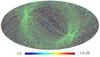
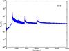
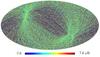
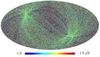
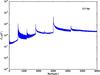
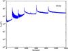
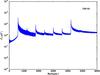
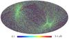
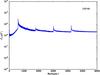
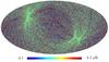
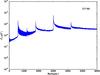
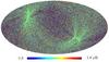
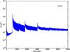
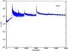
<span style="font-size:150%">'''Section 5.3.10: for convenience, we reproduce here Figures 6, 7 and 8 of Rosset et al.''' </span> | <span style="font-size:150%">'''Section 5.3.10: for convenience, we reproduce here Figures 6, 7 and 8 of Rosset et al.''' </span> | ||
| − | This paper is published as Rosset et al. Planck pre-launch status: High Frequency Instrument polarization calibration. 2010b, A&A, 520, A13 | + | This paper is published as Rosset et al. Planck pre-launch status: High Frequency Instrument polarization calibration. 2010b, A&A, 520, A13 {{PlanckPapers|rosset2010}}. The figures 6, 7 et 8 reproduced hereunder are given in the version on ArXiv 1004.2595 |
| − | The figures 6, 7 et 8 reproduced hereunder are given in the version on ArXiv 1004.2595 | ||
{| border="1" cellpadding="3" cellspacing="0" align="center" style="text-align:centert" width=800px | {| border="1" cellpadding="3" cellspacing="0" align="center" style="text-align:centert" width=800px | ||
Latest revision as of 11:31, 28 November 2017
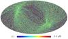
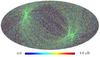
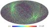
This page is intented to provide complementary figures to those of the 2017 HFI DPC paper (Planck-2020-A3[1]).
Section 5.3.10: for convenience, we reproduce here Figures 6, 7 and 8 of Rosset et al.
This paper is published as Rosset et al. Planck pre-launch status: High Frequency Instrument polarization calibration. 2010b, A&A, 520, A13 Planck-PreLaunch-XIII[2]. The figures 6, 7 et 8 reproduced hereunder are given in the version on ArXiv 1004.2595
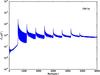
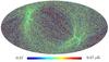
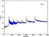
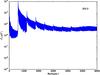
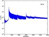
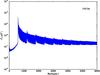
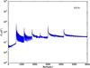
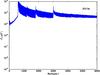
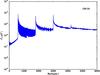
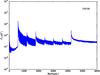
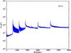
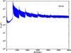
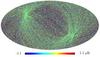
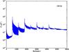
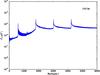
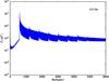
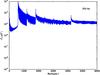
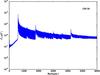
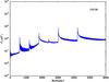
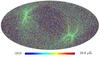
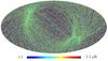
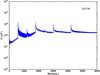
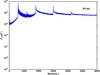
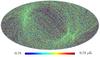
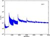
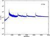
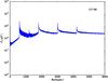
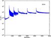
| gain errors (1) | polarization efficiency errors (2) | orientation errors (3) |
|---|---|---|
Error creating thumbnail: convert: unable to extend cache `/tmp/magick-26813EUsxqAk5pq31': File too large @ error/cache.c/OpenPixelCache/4091.
|
Error creating thumbnail: convert: unable to extend cache `/tmp/magick-26820V7rOL4vxSjWL': File too large @ error/cache.c/OpenPixelCache/4091.
|
Error creating thumbnail: convert: unable to extend cache `/tmp/magick-26827aFbx5ldEPIpm': File too large @ error/cache.c/OpenPixelCache/4091.
|
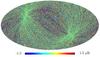
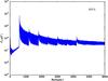
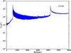
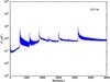
(1) in rms due to gain errors from 0.01% to 1% for E-mode (top) and B-mode (bottom) compared to initial spectrum (solid black lines). Cosmic variance for E-mode is plotted in dashed black line.
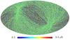
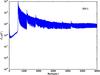
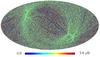
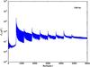
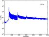
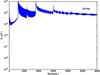
(2) in rms due to polarization efficiency errors from 0.1% to 4% for E-mode (top) and B-mode (bottom) compared to initial spectrum (solid black lines). Cosmic variance for E-mode is plotted in dashed black line.
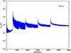
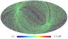
(3) in rms due to various orientation errors from 0.25 to 2 degrees for E-mode (top) and B-mode (bottom) compared to initial spectrum (solid black lines). Cosmic variance for E-mode is plotted in dashed black line.
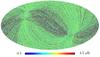
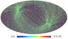
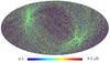
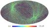
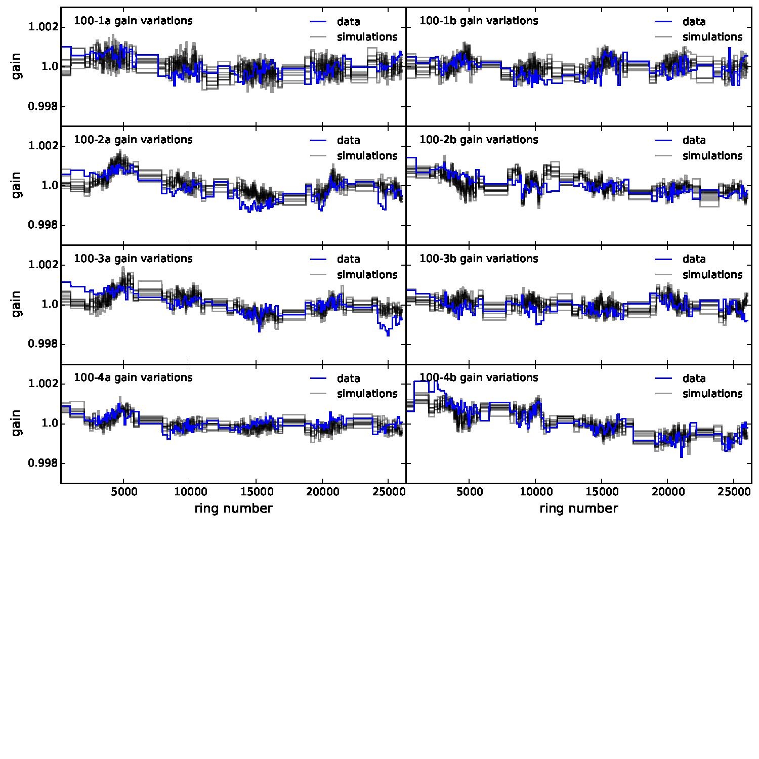
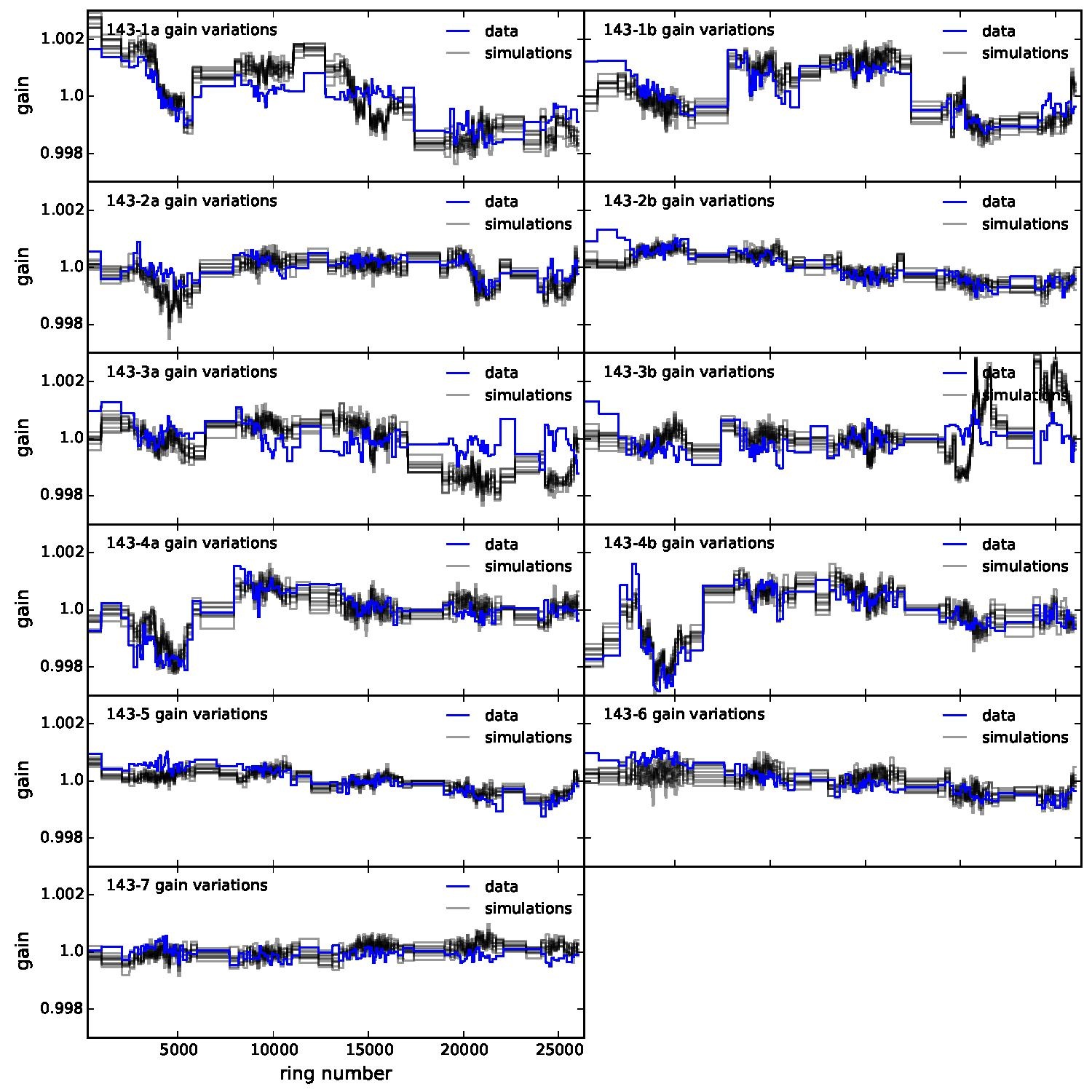
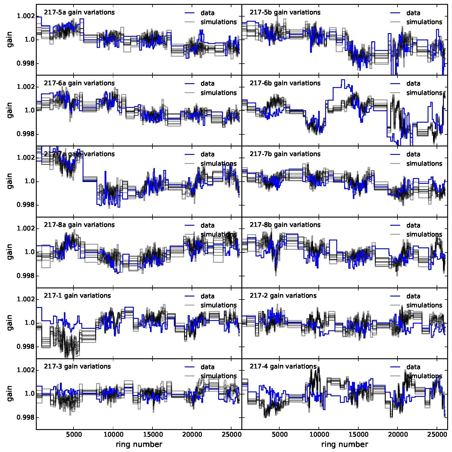
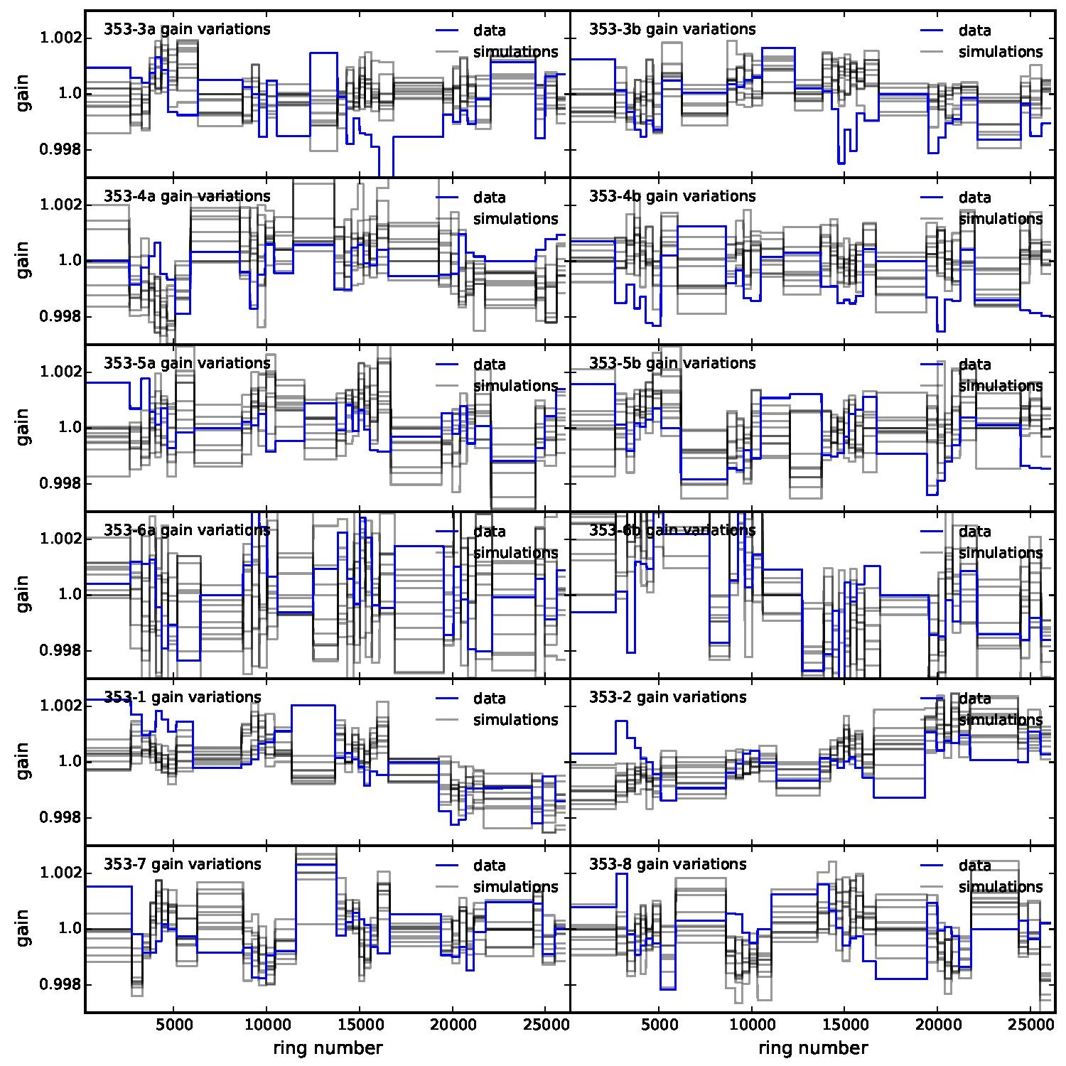
Section 5.5: complementary figures of Fig. 29
| 100 GHz bolometers | 143 GHz bolometers | 217 GHz bolometers | 353 GHz bolometers | ||||
|---|---|---|---|---|---|---|---|
|
|
|
|
|
|
|
|
| 100px | 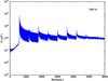
|
|
|
|
|
|
|

|
|
|
|

|
|

|
|
|
|

|
|

|
|
|
|
|
|
|
|

|
|

|
|
|
|

|
|
|
|

|

|
|
|

|
|

|
|
|
|

|
|
|
|
|
|
|
|
| . | . | 
|
|
|
|

|
|
| . | . | 
|
|

|
|
|
|
| . | . | 
|
|

|
|
|
|
| . | . | . | . | 
|
|
|
|
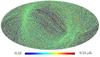
Section 5.13: complementary figures of Fig. 47
| 100 GHz bolometers | 143 GHz bolometers | 217 GHz bolometers | 353 GHz bolometers |
|---|---|---|---|
|
|
|
|
References[edit]
- ↑ Planck 2018 results. III. High Frequency Instrument data processing and frequency maps, Planck Collaboration, 2020, A&A, 641, A3.
- ↑ Planck pre-launch status: High Frequency Instrument polarization calibration, C. Rosset, M. Tristram, N. Ponthieu, et al. , A&A, 520, A13+, (2010).
(Planck) High Frequency Instrument
Data Processing Center
EMI/EMC influence of the 4K cooler mechanical motion on the bolometer readout electronics.
analog to digital converter